Visualizing 2D model data

Section author: Florian Zill (Helmholtz Centre for Environmental Research GmbH - UFZ)

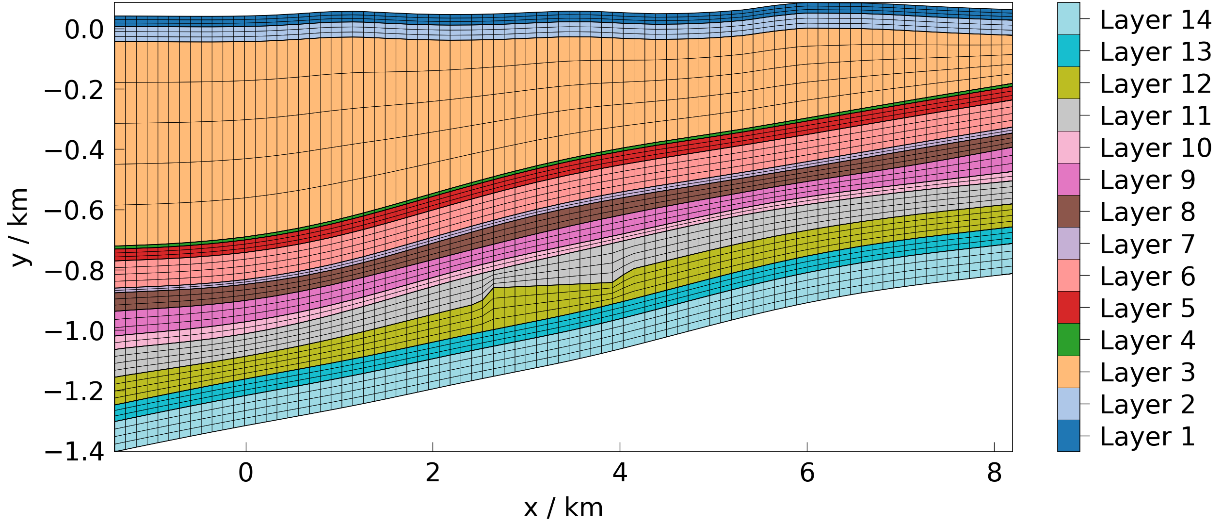
For this example we load a 2D meshseries from within the meshplotlib examples. In the meshplotlib.setup we can provide a dictionary to map names to material ids. First, let’s plot the material ids (cell_data). Per default in the setup, this will automatically show the element edges.

import ogstools.meshplotlib as mpl
from ogstools.meshplotlib.examples import meshseries_THM_2D
from ogstools.propertylib import presets

mpl.setup.reset()
mpl.setup.length.output_unit = "km"
mpl.setup.material_names = {i + 1: f"Layer {i+1}" for i in range(26)}
mesh = meshseries_THM_2D.read(1)

To read your own data as a mesh series you can do:

from ogstools.meshlib import MeshSeries
mesh_series = MeshSeries("filepath/filename_pvd_or_xdmf")

fig = mpl.plot(mesh, presets.material_id)

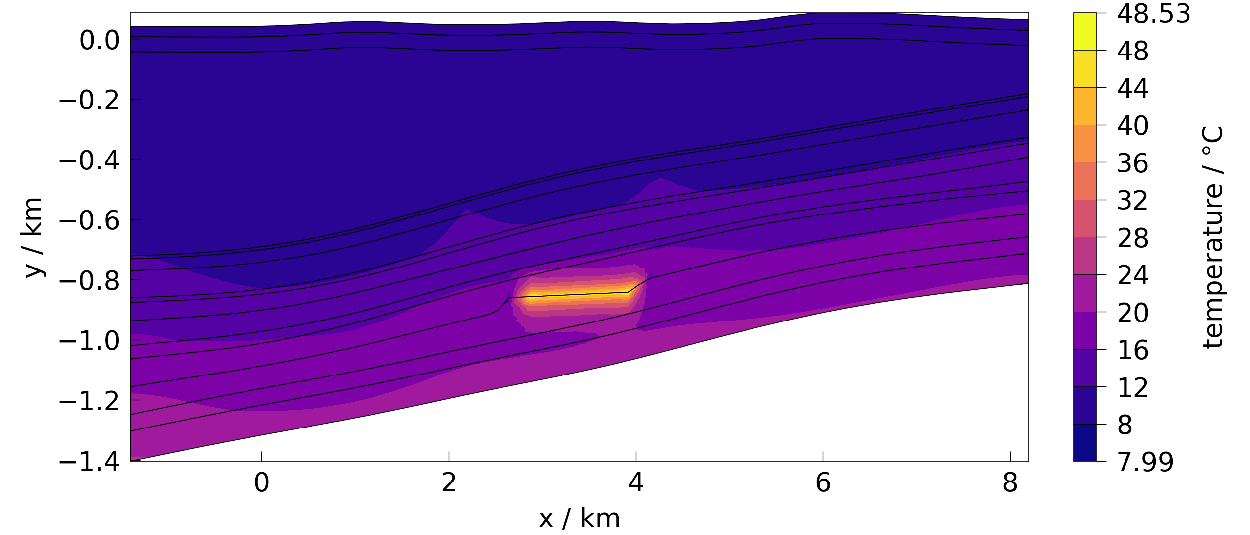
Now, let’s plot the temperature field (point_data) at the first timestep. The default temperature property from the propertylib reads the temperature data as Kelvin and converts them to degrees Celsius.

fig = mpl.plot(mesh, presets.temperature)

We can also plot components of vector properties:

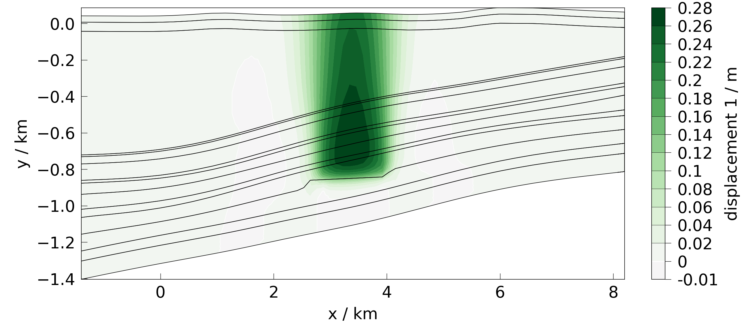
fig = mpl.plot(mesh, presets.displacement[0])

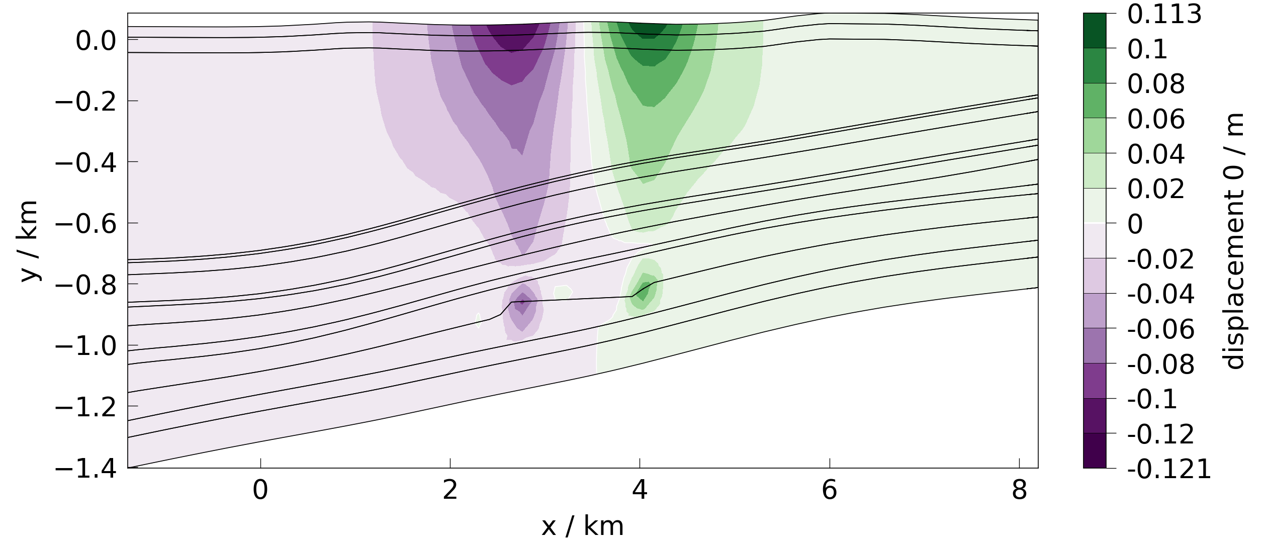
fig = mpl.plot(mesh, presets.displacement[1])

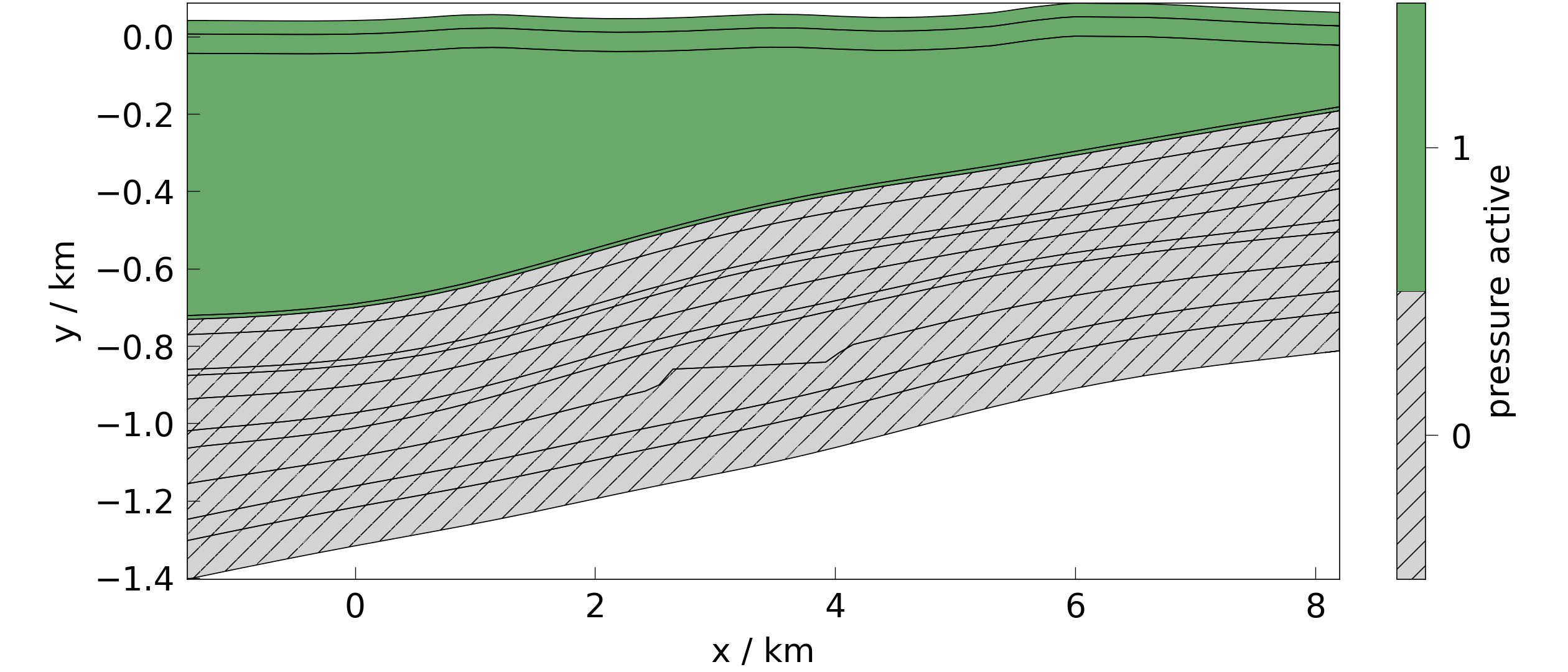
This example has hydraulically deactivated subdomains:

fig = mpl.plot(mesh, presets.pressure.get_mask())

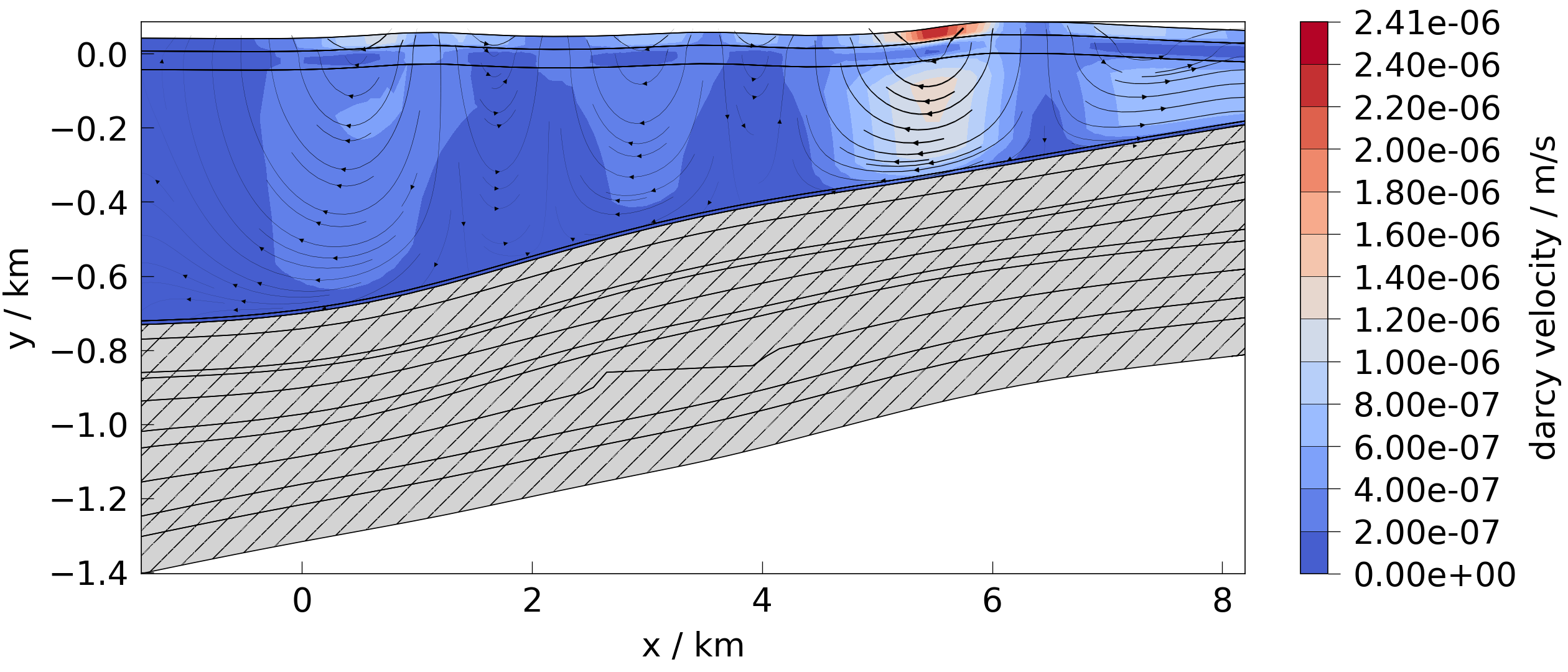
Let’s plot the fluid velocity field.

fig = mpl.plot(mesh, presets.velocity)

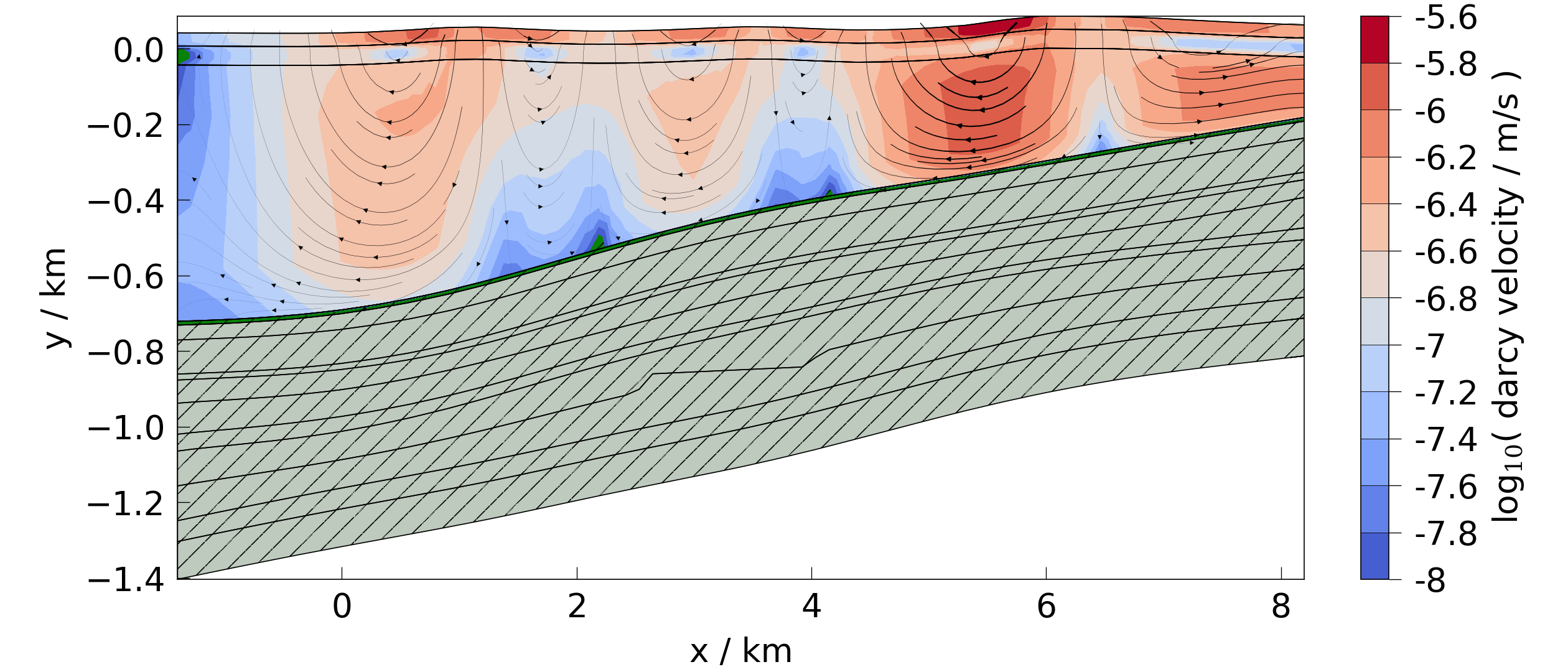
Let’s plot it again, this time log-scaled.

mpl.setup.log_scaled = True
mpl.setup.p_min = -8
fig = mpl.plot(mesh, presets.velocity)