Visualizing 2D model data

To demonstrate the creation of filled contour plots we load a 2D THM meshseries example. In the plot.setup we can provide a dictionary to map names to material ids. Other plot configurations are also available, see: ogstools.plot.plot_setup.PlotSetup. Some of these options are also available as keyword arguments in the function call. Please see ogstools.plot.contourplots.contourf for more information.

import ogstools as ot
from ogstools import examples

ot.plot.setup.material_names = {i + 1: f"Layer {i+1}" for i in range(26)}
ms = examples.load_meshseries_THM_2D_PVD().scale(spatial="km")
mesh = ms.mesh(1)

To read your own data as a mesh series you can do:

mesh_series = ot.MeshSeries("filepath/filename_pvd_or_xdmf", "km")

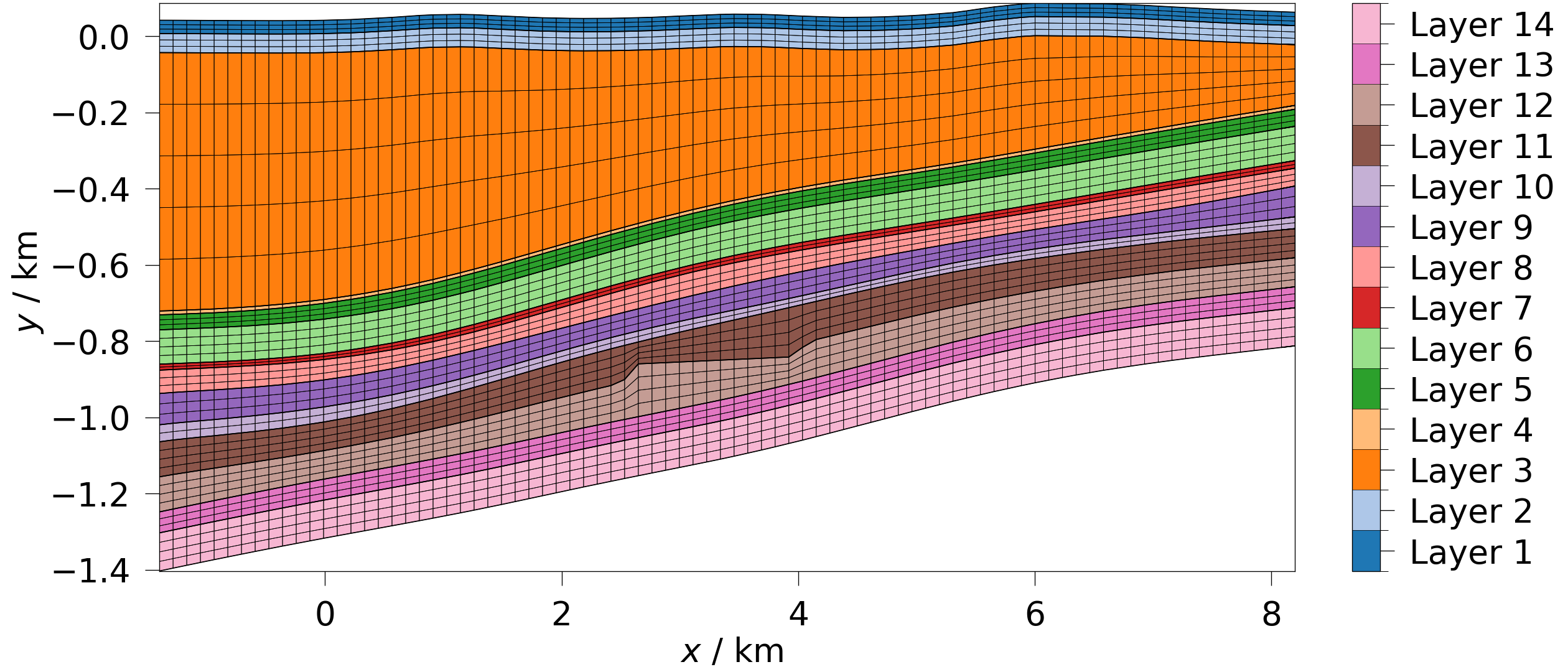
Plotting Cell Data

First, let’s plot the material ids, which is part of the mesh’s cell_data. Per default in the setup, this will automatically show the element edges.

fig = ot.plot.contourf(mesh, ot.variables.material_id)

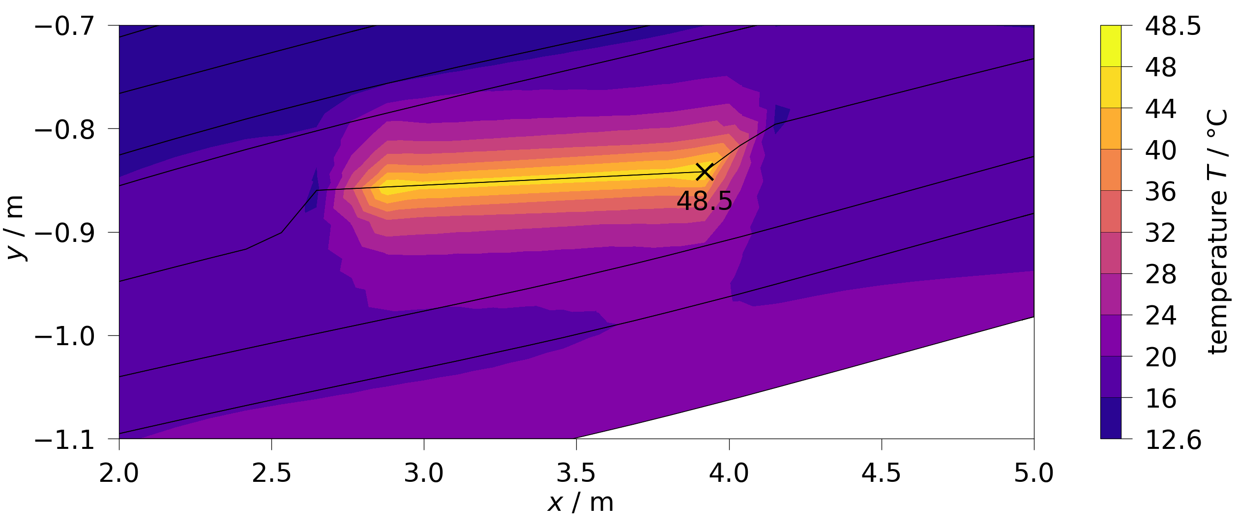
Plotting Point Data

Now, let’s plot the temperature field (point_data) at the first timestep. The default temperature variable from the variables reads the temperature data as Kelvin and converts them to degrees Celsius. This also shows how to only plot a specific part of the model by creating a clip with pyvista.clip_box beforehand.

part = mesh.clip_box(bounds=[2, 5, -1.1, -0.7, 6, 7], invert=False)
fig = ot.plot.contourf(part, ot.variables.temperature, show_max=True)

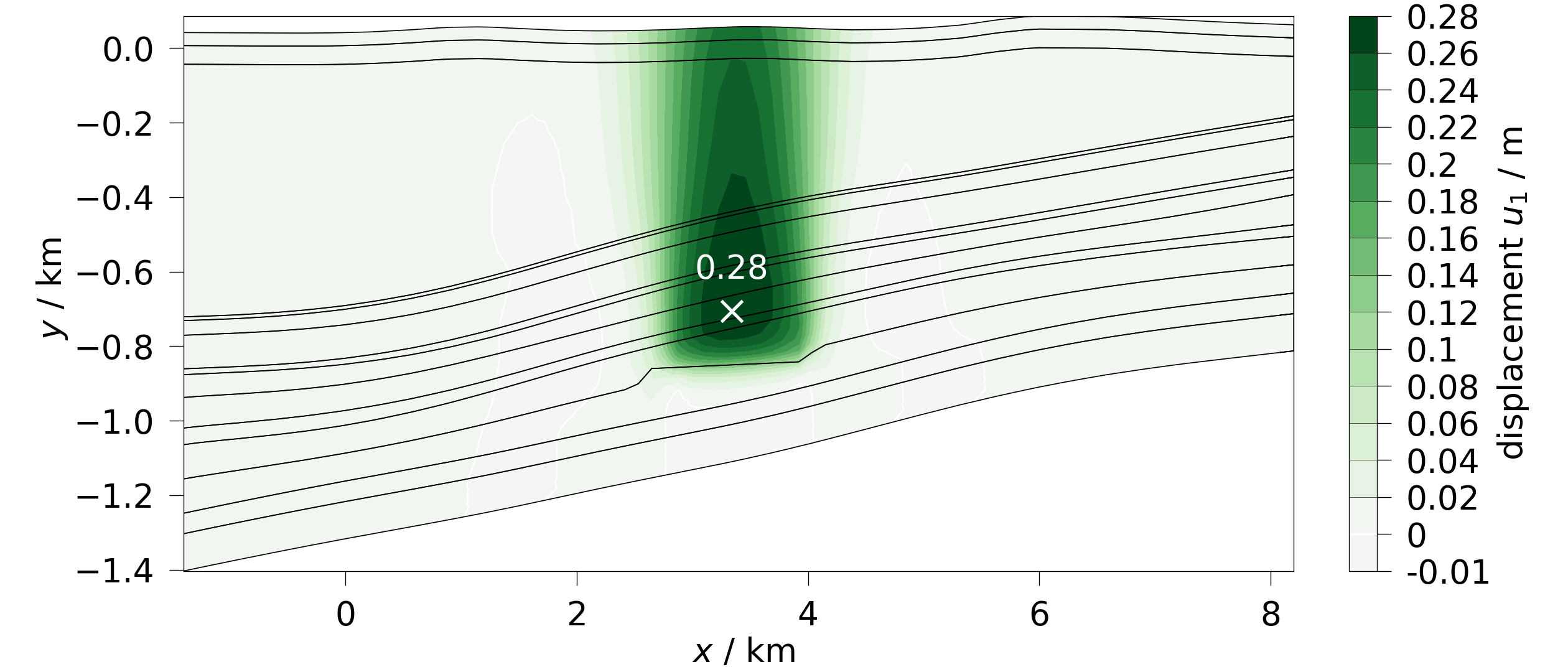
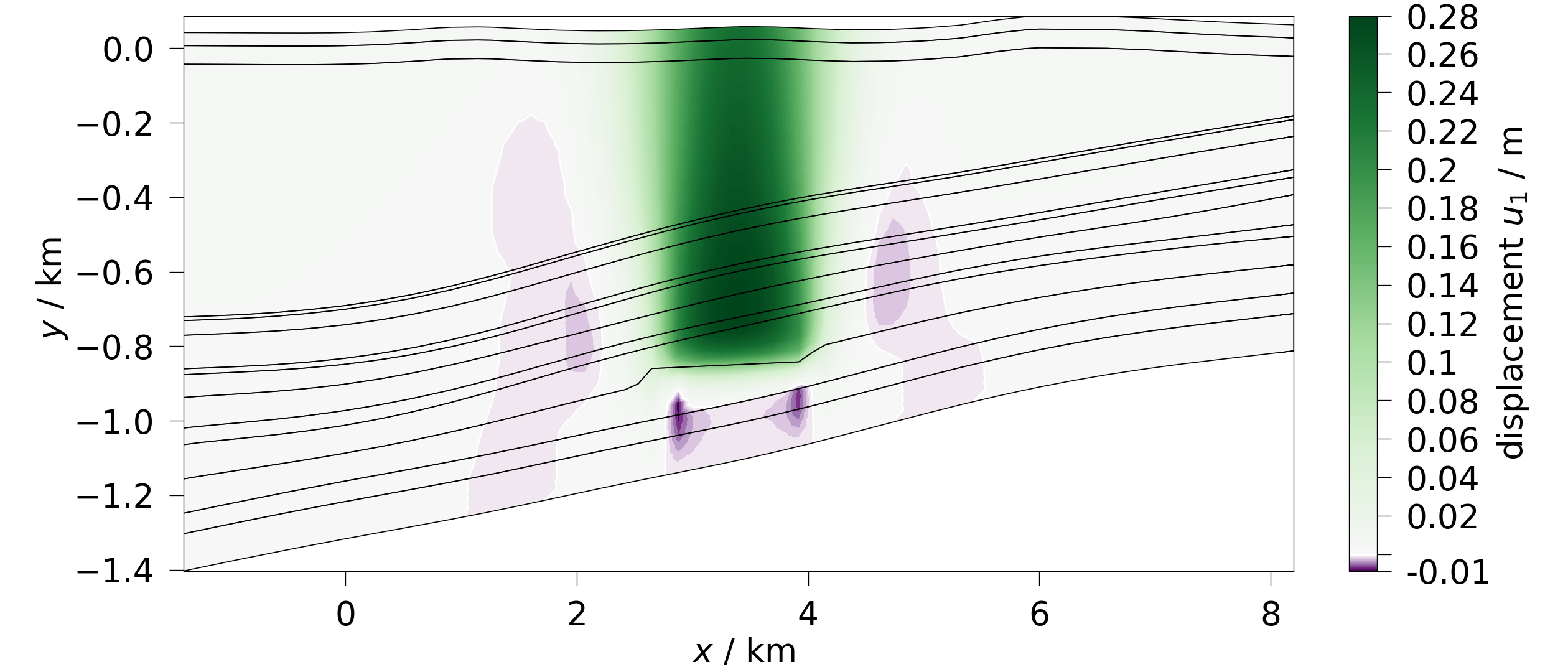
We can also plot components of vector variables:

fig = ot.plot.contourf(
    mesh, ot.variables.displacement[0], show_min=True, show_max=True
)

fig = ot.plot.contourf(mesh, ot.variables.displacement[1], show_max=True)

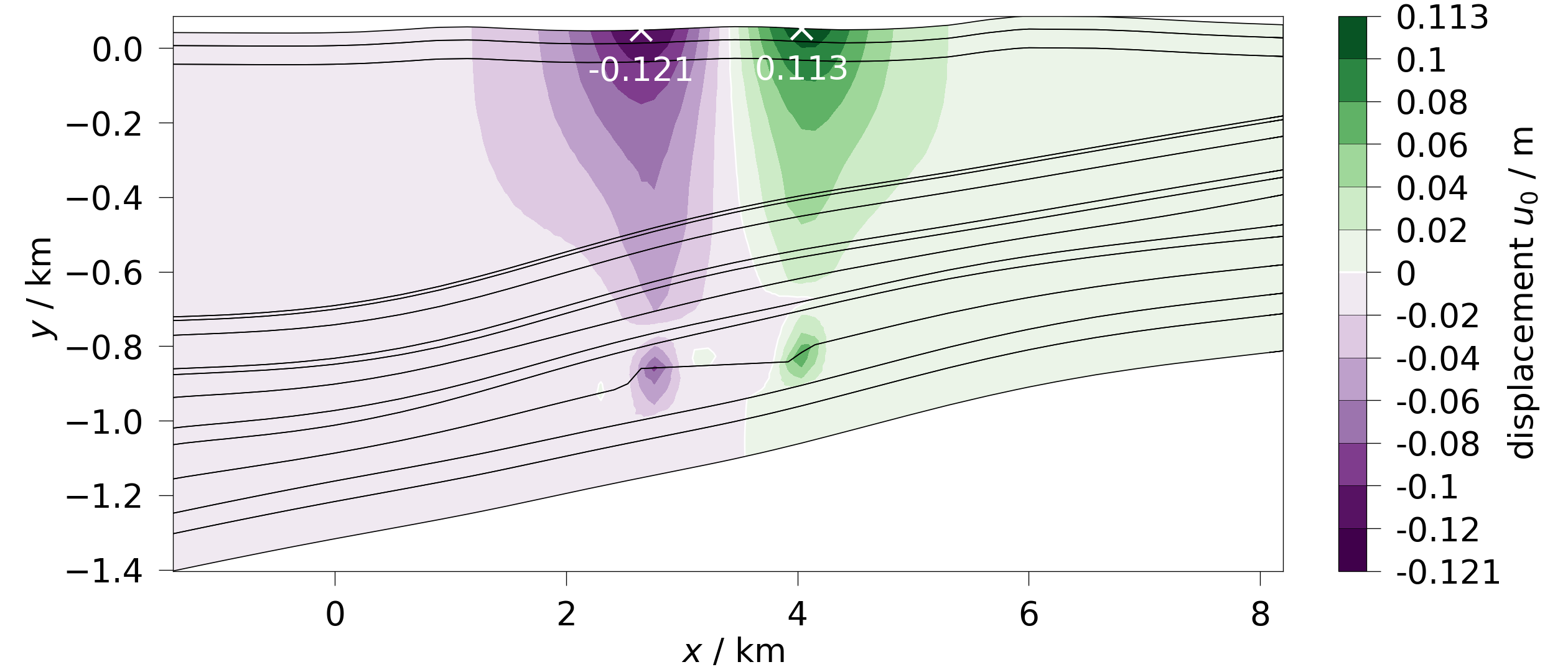
To have a continuous colormap instead of discrete colors per level pass a the equally named argument. In this case this helps to increase the level of detail of the negative displacements due to the bilinear colormap.

fig = ot.plot.contourf(mesh, ot.variables.displacement[1], continuous_cmap=True)

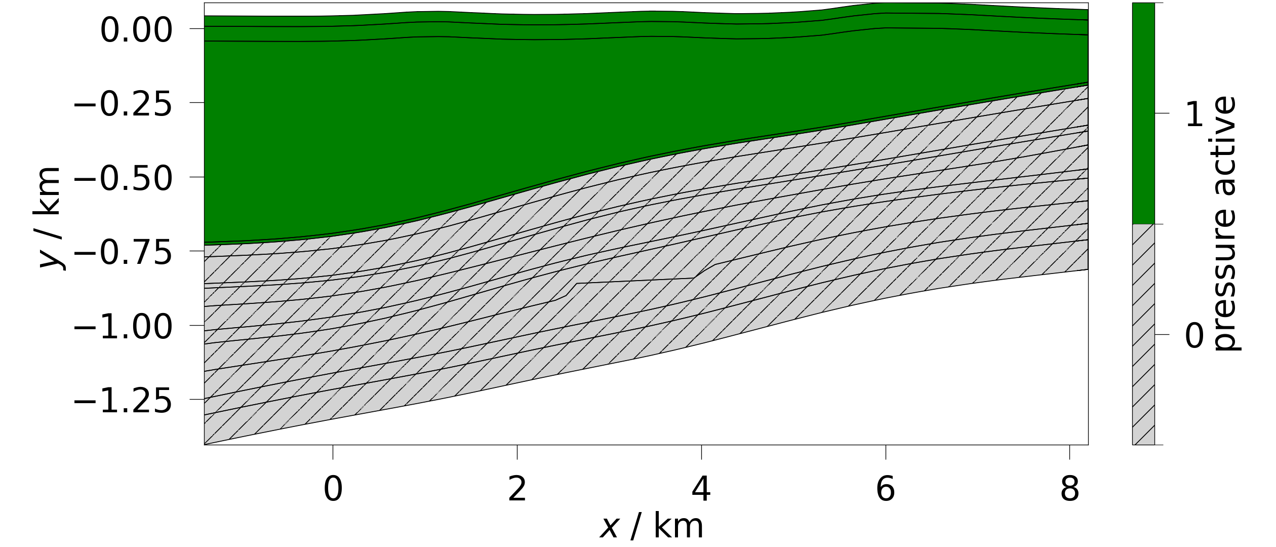
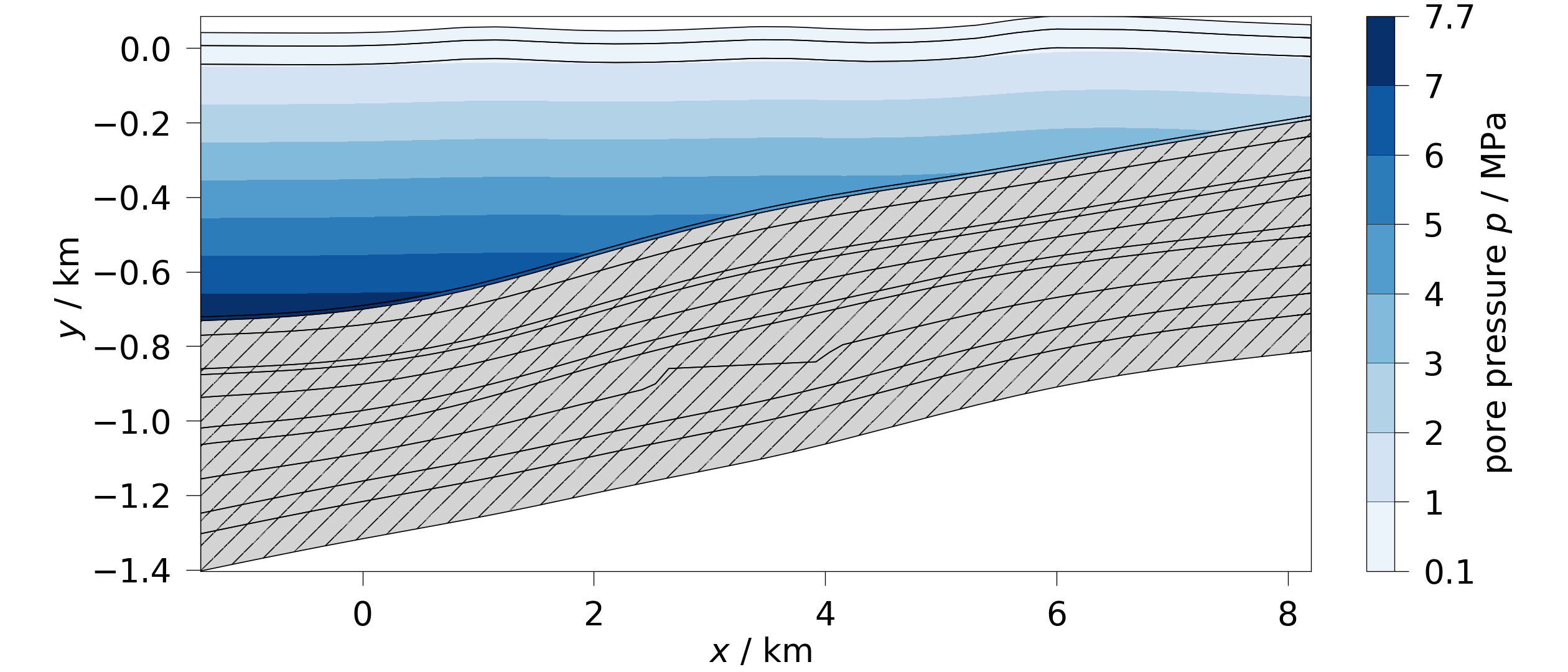
Plotting with deactivated subdomains

This example has hydraulically deactivated subdomains, which will mask the related variables.

fig = ot.plot.contourf(mesh, ot.variables.pressure.get_mask(), fontsize=40)

fig = ot.plot.contourf(mesh, ot.variables.pressure)

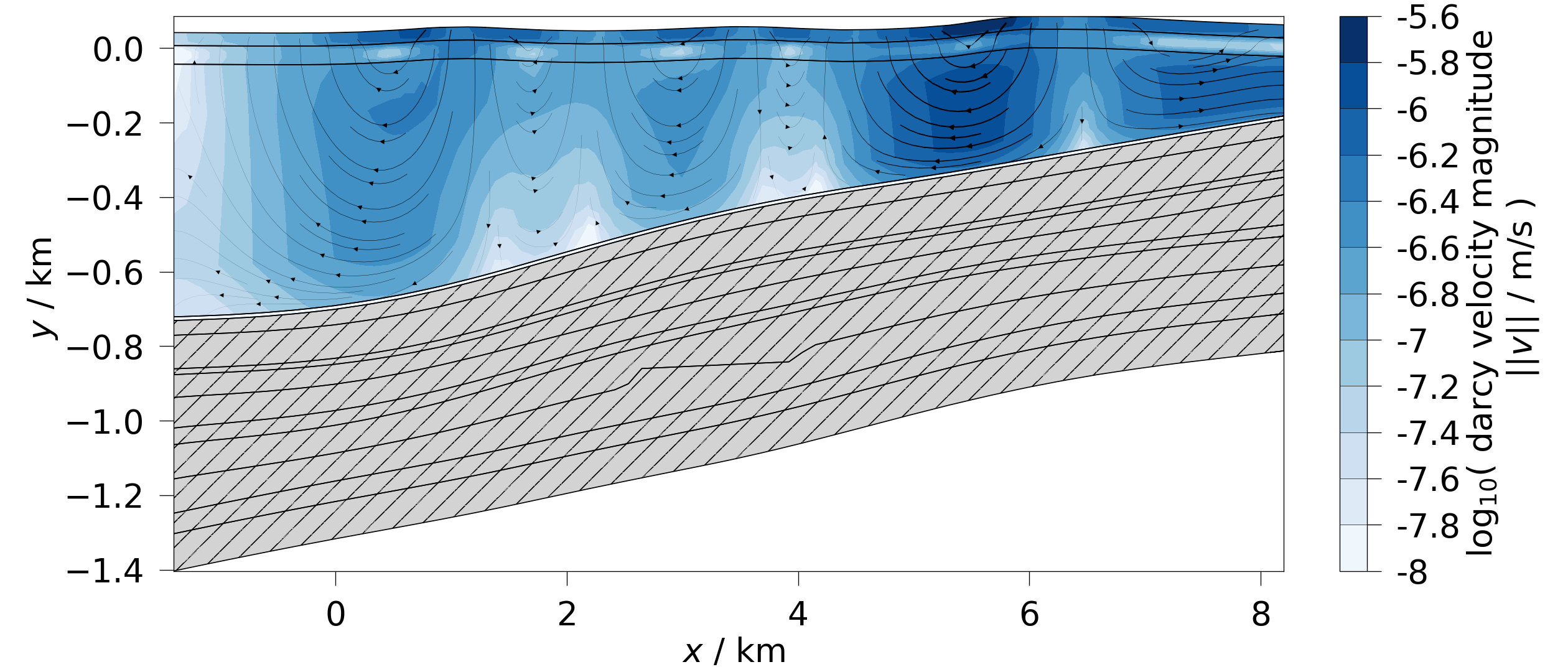
Plotting vector data

Let’s plot the fluid velocity field. As this is vectorial data, this will automatically add streamlines to indicate the vector directions.

fig = ot.plot.contourf(mesh, ot.variables.velocity, show_region_bounds=False)

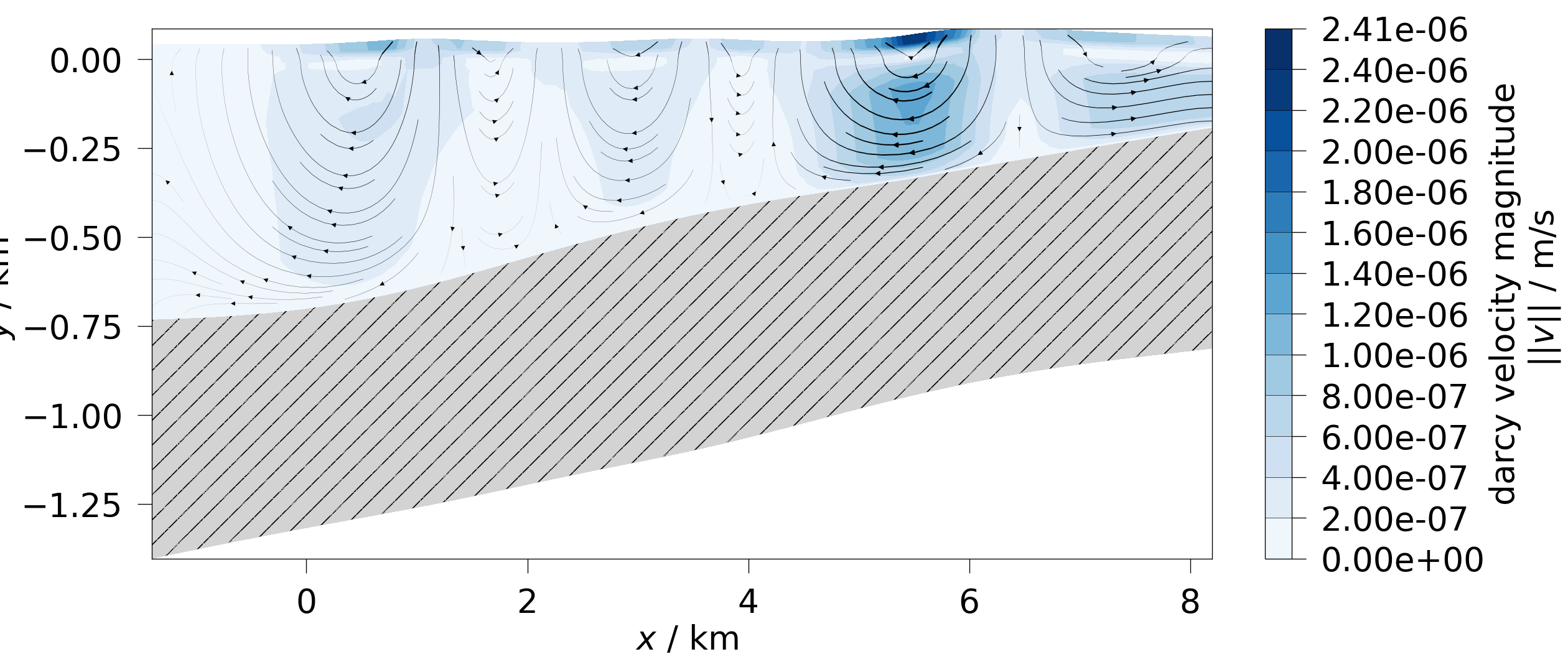
Let’s plot it again, this time log-scaled.

fig = ot.plot.contourf(mesh, ot.variables.velocity, log_scaled=True, vmin=-8)