Note
Go to the end to download the full example code.
Extract a 1D profile from 2D and plot it#
Section author: Feliks Kiszkurno (Helmholtz Centre for Environmental Research GmbH - UFZ)
For this example we load a 2D meshseries from within the meshplotlib
examples. In the meshplotlib.setup we can provide a dictionary to map names
to material ids. First, let’s plot the material ids (cell_data). Per default in
the setup, this will automatically show the element edges.
0. Setup and imports#
import matplotlib.pyplot as plt
import numpy as np

import ogstools.meshplotlib as mpl
from ogstools import examples
from ogstools.meshlib import sample_polyline
from ogstools.meshplotlib import lineplot, plot_profile
from ogstools.propertylib import Scalar, properties

mpl.setup.reset()
mpl.setup.combined_colorbar = False
plt.rcdefaults()
# mpl.setup.length.output_unit = "km"
1. Single fracture#
Define profile line by providing a list of points in an X, Y, Z coordinates and loading an example data set:
ms_HT = examples.load_meshseries_HT_2D_XDMF()

profile_HT = np.array([[4, 2, 0], [4, 18, 0]])
ms_HT_sp, ms_HT_kp = sample_polyline(
    ms_HT.read(-1),
    ["pressure", "temperature"],
    profile_HT,
)
It has returned a DataFrame containing all information about profile and numpy array with position of the “knot-points”. Let’s investigate the DataFrame first:
ms_HT_sp.head(10)
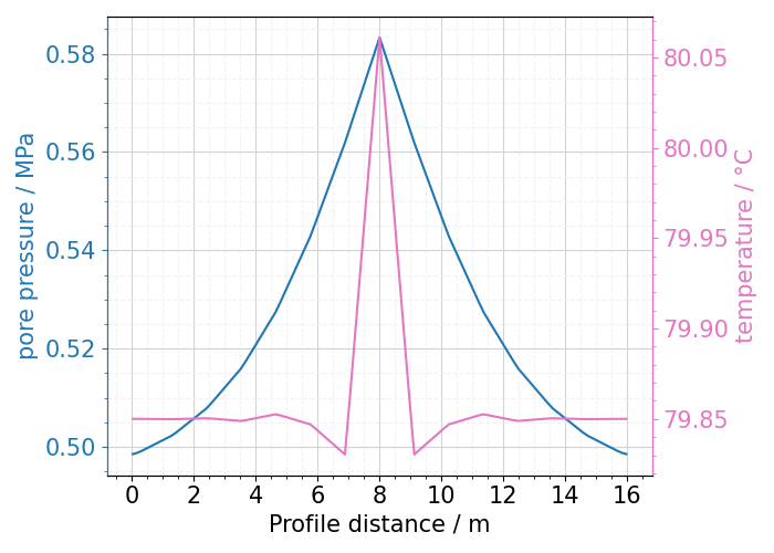
We can see the spatial coordinates of points on the profile (“x”, “y”, “z” - columns), distances from the beginning of the profile (“dist”) and within current segment (“dist_in_segment”). Note, that since we defined our profile on only two points, there is only one segment, hence in this special case columns dist and dist_in_segment are identical. At the end of the DataFrame we can can find two columns with the properties that we are interested in: “temperature” and “pressure”. Each occupies one column, as those are scalar values. Using columns “dist”, “pressure” and “temperature” we can easily plot the data:
fig, ax = plt.subplots(1, 1, figsize=(7, 5))
ax = lineplot(
    x="dist",
    y=["pressure", "temperature"],
    mesh=ms_HT.read(-1),
    profile_points=profile_HT,
    ax=ax,
    twinx=True,
    fontsize=15,
)
fig.tight_layout()

What happens when we are interested in vector property? We can see it in the following example using Darcy velocity:
ms_HT_sp, ms_HT_kp = sample_polyline(
    ms_HT.read(-1),
    "darcy_velocity",
    profile_HT,
)
ms_HT_sp.head(5)
Now we have two columns for the property. Darcy velocity is a vector, therefore “sample_over_polyline” has split it into two columns and appended the property name with increasing integer. Note, that this suffix has no physical meaning and only indicates order. It is up to user to interpret it in a meaningful way. By the OpenGeoSys conventions, “darcy_velocity_0” will be in the x-direction and “darcy_velocity_1” in y-direction.
2. Elder benchmark#
In this example we will provide a Scalar object from the propertylib to define the property of interest. “sample_over_polyline” will automatically convert the data from “data_unit” to “output_unit”:
profile_CT = np.array(
    [
        [47.0, 1.17, 72.0],  # Point A
        [-4.5, 1.17, -59.0],  # Point B
    ]
)

ms_CT = examples.load_meshseries_CT_2D_XDMF()

si = Scalar(
    data_name="Si", data_unit="", output_unit="%", output_name="Saturation"
)
ms_CT_sp, ms_CT_kp = sample_polyline(
    ms_CT.read(11),
    si,
    profile_CT,
)
As before we can see the profile parameters and properties values in a DataFrame:
ms_CT_sp.head(5)
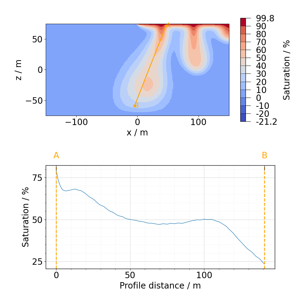
This time we will prepare more complicated plot showing both mesh data and the profile.
fig, ax = plot_profile(
    ms_CT.read(11),
    si,
    profile_CT,
    resolution=100,
    profile_plane=[0, 2],  # This profile is in XZ plane, not XY!
)
fig, ax = mpl.update_font_sizes(label_axes="none", fig=fig)
fig.tight_layout()

3. THM#
It is also possible to obtain more than one property at the same time using more complex profiles. They can be constructed by providing more than 2 points. With those points:
profile_THM = np.array(
    [
        [-1000.0, -175.0, 6700.0],  # Point A
        [-600.0, -600.0, 6700.0],  # Point B
        [100.0, -300.0, 6700.0],  # Point C
        [910.0, -590.0, 6700.0],  # Point D
    ]
)

profile_THM = np.array(
    [
        [-1000.0, -175.0, 6700.0],  # Point A
        [-600.0, -600.0, 6700.0],  # Point B
        [100.0, -300.0, 6700.0],  # Point C
        [3500, -900.0, 6700.0],  # Point D
    ]
)
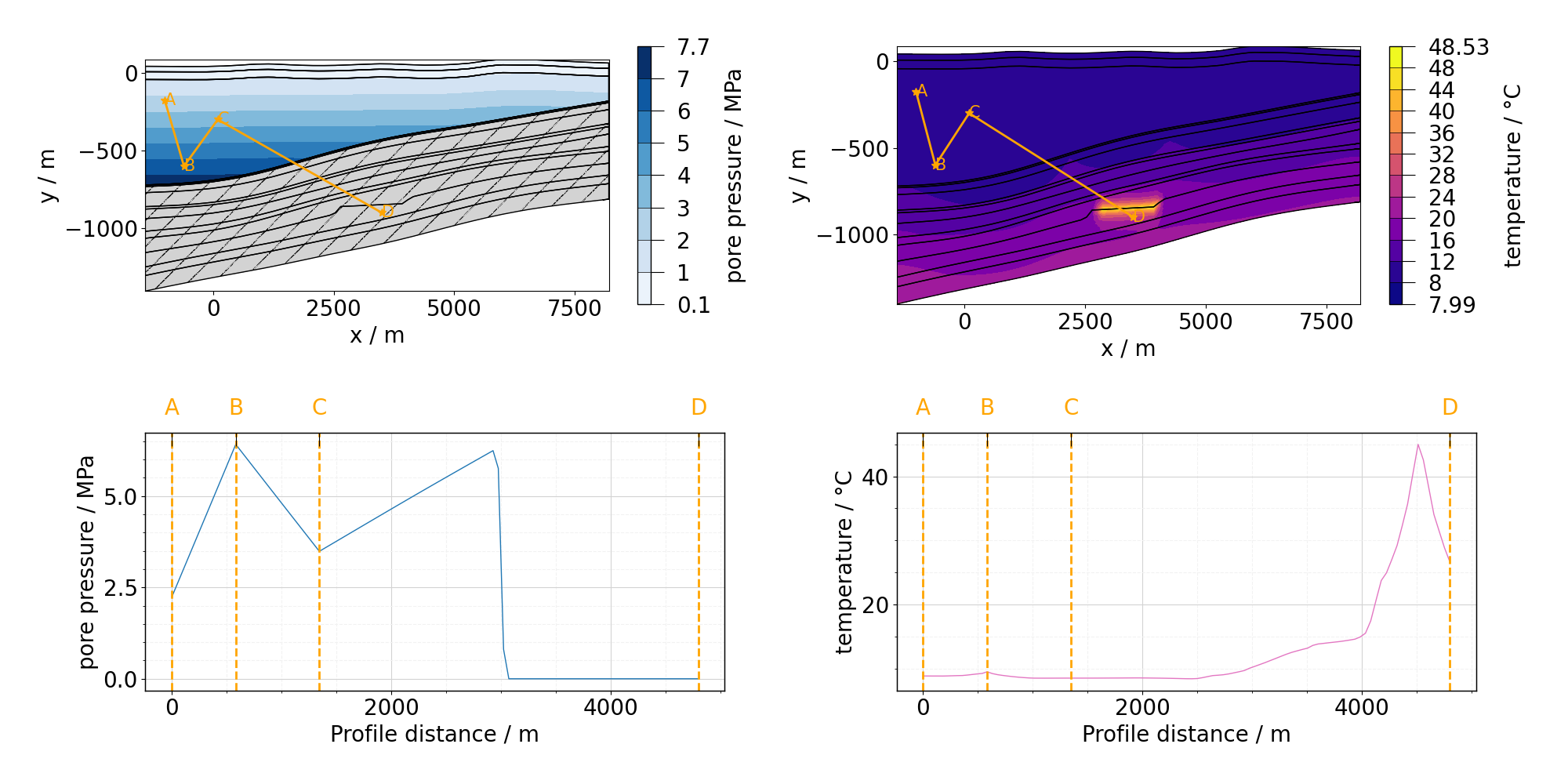
the profile will run as follows:
Point B will at the same time be the last point in the first segment AB and first one in second segment BC, however in the returned array, it will occur only once. For this example we will use a different dataset:
meshseries_THM = examples.load_meshseries_THM_2D_PVD()
ms_THM_sp, dist_at_knot = sample_polyline(
    meshseries_THM.read(-1),
    [properties.pressure, properties.temperature],
    profile_THM,
    resolution=100,
)
Again, we can investigate the returned DataFrame, but this time we will have a look at its beginning:
ms_THM_sp.head(5)
and end:
ms_THM_sp.tail(10)
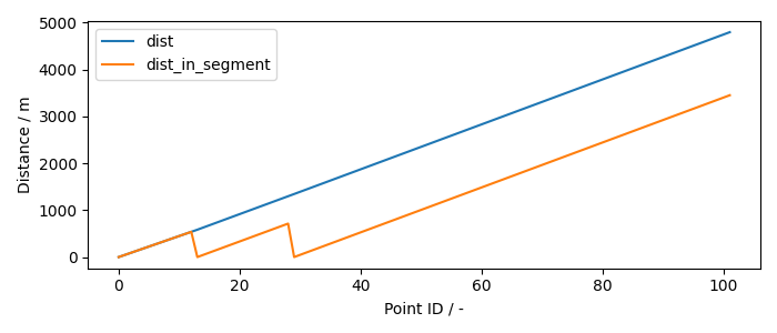
Note, that unlike in the first example, here the columns “dist” and “dist_in_segment” are not identical, as this time profile consists of multiple segments. Following figure illustrates the difference:
plt.rcdefaults()
fig, ax = plt.subplots(1, 1, figsize=(7, 3))
ax.plot(ms_THM_sp["dist"], label="dist")
ax.plot(ms_THM_sp["dist_in_segment"], label="dist_in_segment")
ax.set_xlabel("Point ID / -")
ax.set_ylabel("Distance / m")
ax.legend()
fig.tight_layout()

Orange line returns to 0 twice. It is because of how the overlap of nodal points between segments is handled. Nodal point always belongs to the segment it starts: point B is included in segment BC but not AB and point C in CD but not in in BC. Following figure shows the profile on the mesh:
plt.rcdefaults()
fig, ax = plot_profile(
    meshseries_THM.read(-1),
    [properties.pressure, properties.temperature],
    profile_THM,
    resolution=100,
)
fig, ax = mpl.update_font_sizes(label_axes="none", fig=fig)
fig.tight_layout()

Total running time of the script: (0 minutes 2.747 seconds)
