Note
Go to the end to download the full example code.
How to plot data at observation points#
Section author: Florian Zill (Helmholtz Centre for Environmental Research GmbH - UFZ)
In this example we plot the data values on observation points over all
timesteps. Since requested observation points don’t necessarily coincide with
actual nodes of the mesh different interpolation options are available. See
ogstools.meshlib.mesh_series.MeshSeries.probe for more details.
Here we use a component transport example from the ogs benchmark gallery
(https://www.opengeosys.org/docs/benchmarks/hydro-component/elder/).
import matplotlib.pyplot as plt
import numpy as np

from ogstools import examples, meshplotlib
from ogstools.meshplotlib.utils import justified_labels
from ogstools.propertylib import Scalar

meshplotlib.setup.reset()
mesh_series = examples.load_meshseries_CT_2D_XDMF()
si = Scalar(
    data_name="Si", data_unit="", output_unit="%", output_name="Saturation"
)
To read your own data as a mesh series you can do:
from ogstools.meshlib import MeshSeries
mesh_series = MeshSeries("filepath/filename_pvd_or_xdmf")
You can also use a property from the available presets instead of needing to create your own: Property Presets
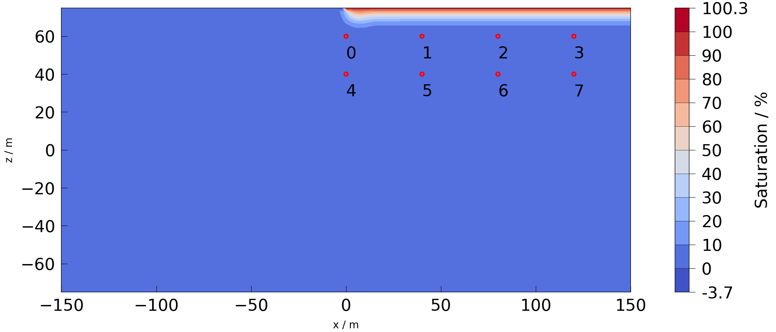
Let’s define 4 observation points and plot them on the mesh.
points = np.asarray(
    [[x, 0, 60] for x in [0, 40, 80, 120]]
    + [[x, 0, 40] for x in [0, 40, 80, 120]]
)
fig = meshplotlib.plot(mesh_series.read(0), si)
fig.axes[0].scatter(points[:, 0], points[:, 2], s=50, fc="none", ec="r", lw=3)
for i, point in enumerate(points):
    fig.axes[0].annotate(str(i), (point[0], point[2] - 5), va="top")
plt.rcdefaults()

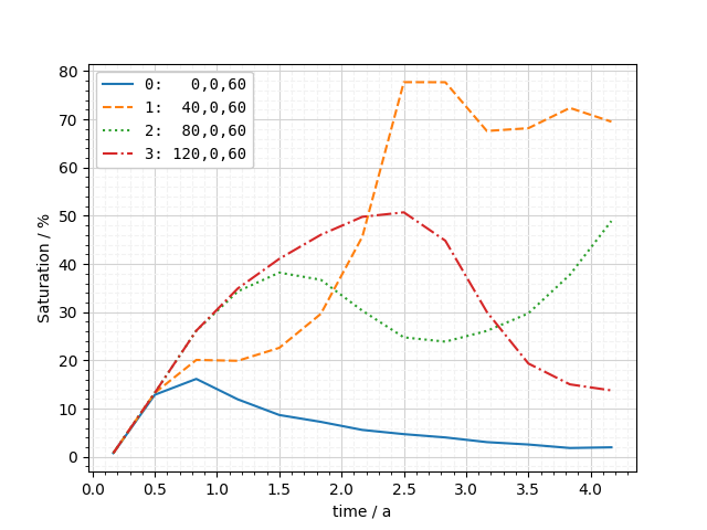
And now probe the points and the values over time:
labels = [f"{i}: {label}" for i, label in enumerate(justified_labels(points))]
fig = meshplotlib.plot_probe(
    mesh_series=mesh_series, points=points[:4], mesh_property=si,
    time_unit="a", labels=labels[:4]
)

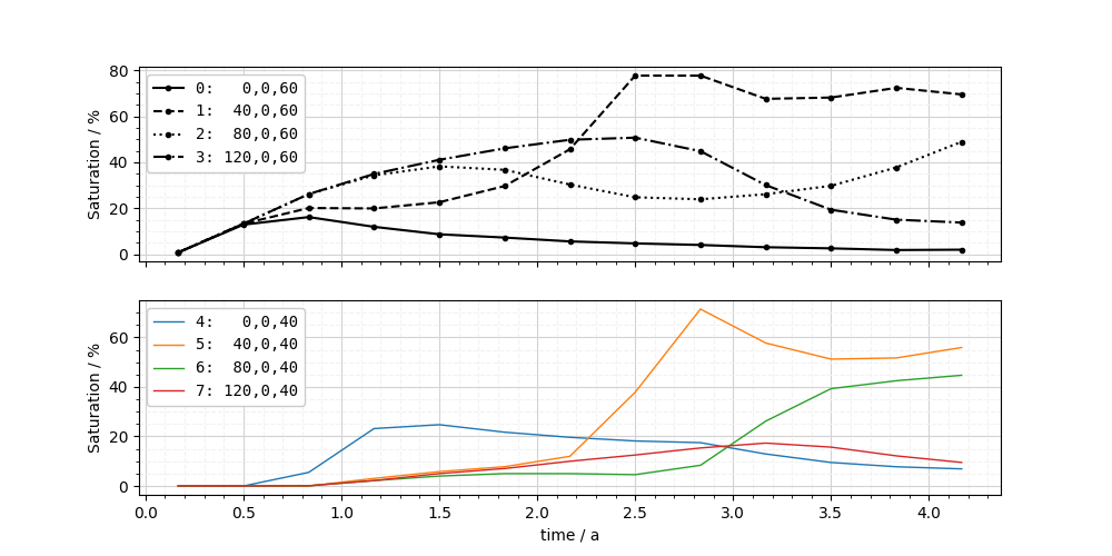
You can also pass create your own matplotlib figure and pass the axes object. Additionally, you can pass any keyword arguments which are known by matplotlibs plot function to further customize the curves. In this case marker and linewidth are not part of the API of plot_probe but get processed correctly anyway.
fig, axs = plt.subplots(nrows=2, figsize=[10, 5])
meshplotlib.plot_probe(
    mesh_series, points[:4], si, time_unit="a", ax=axs[0], colors=["k"],
    labels=labels[:4], marker=".")
meshplotlib.plot_probe(
    mesh_series, points[4:], si, time_unit="a", ax=axs[1], linestyles=["-"],
    labels=labels[4:], linewidth=1,
)

Total running time of the script: (0 minutes 1.352 seconds)
