Feflowlib: How to modify boundary conditions after conversion of a FEFLOW model.

Section author: Julian Heinze (Helmholtz Centre for Environmental Research GmbH - UFZ)

This example shows how boundary conditions can be modified after converting a FEFLOW model. First we will change the values of the boundary conditions and later we will show how to define a new boundary mesh.

0. Necessary imports

import tempfile
from pathlib import Path

import numpy as np
import pyvista as pv

import ogstools as ot
from ogstools.examples import feflow_model_2D_HT
from ogstools.feflowlib import assign_bulk_ids

1. Load a FEFLOW model (.fem) as a FeflowModel object to further work it. During the initialisation, the FEFLOW file is converted.

temp_dir = Path(tempfile.mkdtemp("converted_models"))
feflow_model = ot.FeflowModel(feflow_model_2D_HT, temp_dir / "HT_model")
mesh = feflow_model.mesh
# Print information about the mesh.
print(mesh)

UnstructuredGrid (0x7b26fcde4160)
  N Cells:    6260
  N Points:   3228
  X Bounds:   -2.500e+02, 9.000e+02
  Y Bounds:   3.500e+02, 6.500e+02
  Z Bounds:   0.000e+00, 0.000e+00
  N Arrays:   34

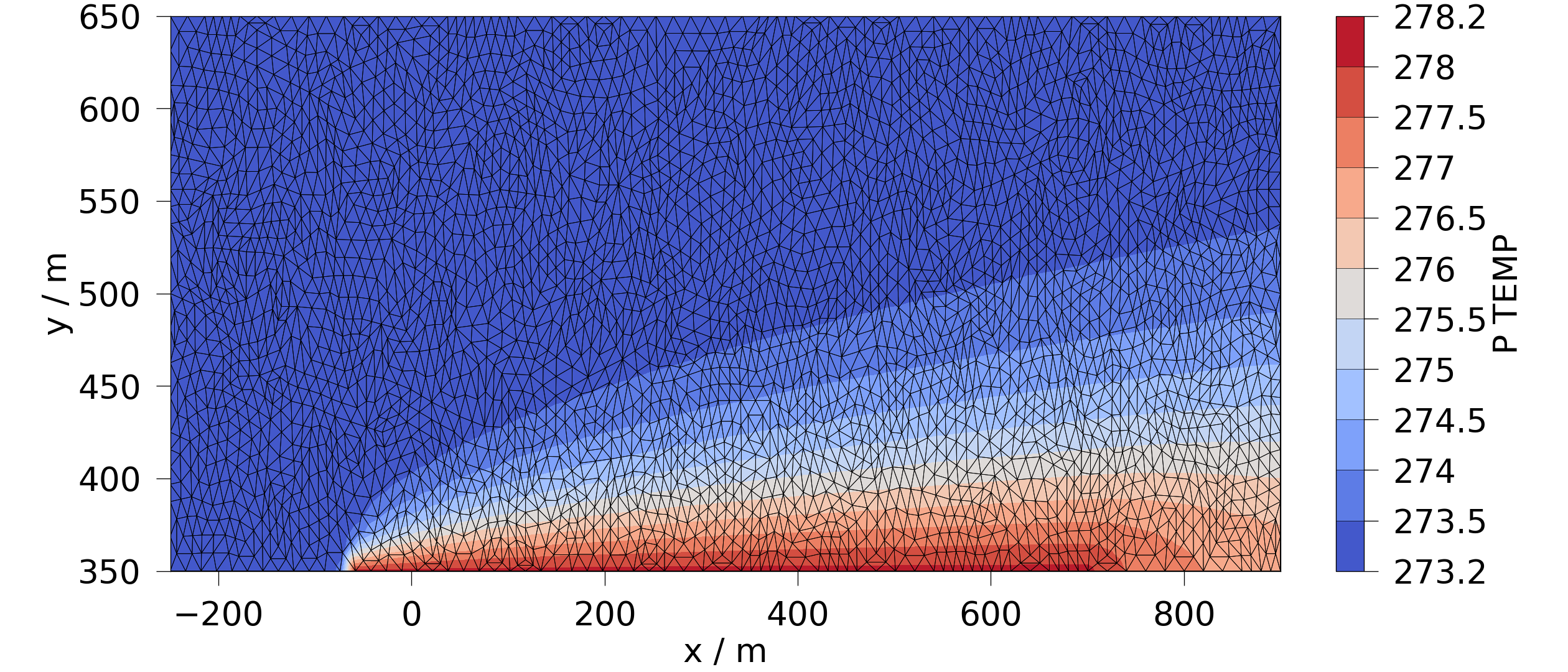
2. Plot the temperature simulated in FEFLOW on the mesh.

fig = ot.plot.contourf(mesh, "P_TEMP", show_edges=True)

3. As the FEFLOW data now are a pyvista.UnstructuredGrid, all pyvista functionalities can be applied to it. Further information can be found at https://docs.pyvista.org/version/stable/user-guide/simple.html. For example it can be saved as a VTK Unstructured Grid File (*.vtu). This allows to use the FEFLOW model for OGS simulation or to observe it in Paraview`.

pv.save_meshio(temp_dir / "HT_mesh.vtu", mesh)

4. Run the FEFLOW model in OGS.

feflow_model.setup_prj(end_time=1e11, time_stepping=[(1, 1e10)])
feflow_model.run()
ms = ot.MeshSeries(temp_dir / "HT_model.pvd")

OGS finished with project file /tmp/tmpeim6fyw1converted_models/HT_model.prj.
Execution took 1.472346544265747 s
Project file written to output.

5. Plot the temperature simulated in OGS.

ogs_sim_res = ms.mesh(ms.timesteps[-1])
ot.plot.contourf(ogs_sim_res, ot.variables.temperature)

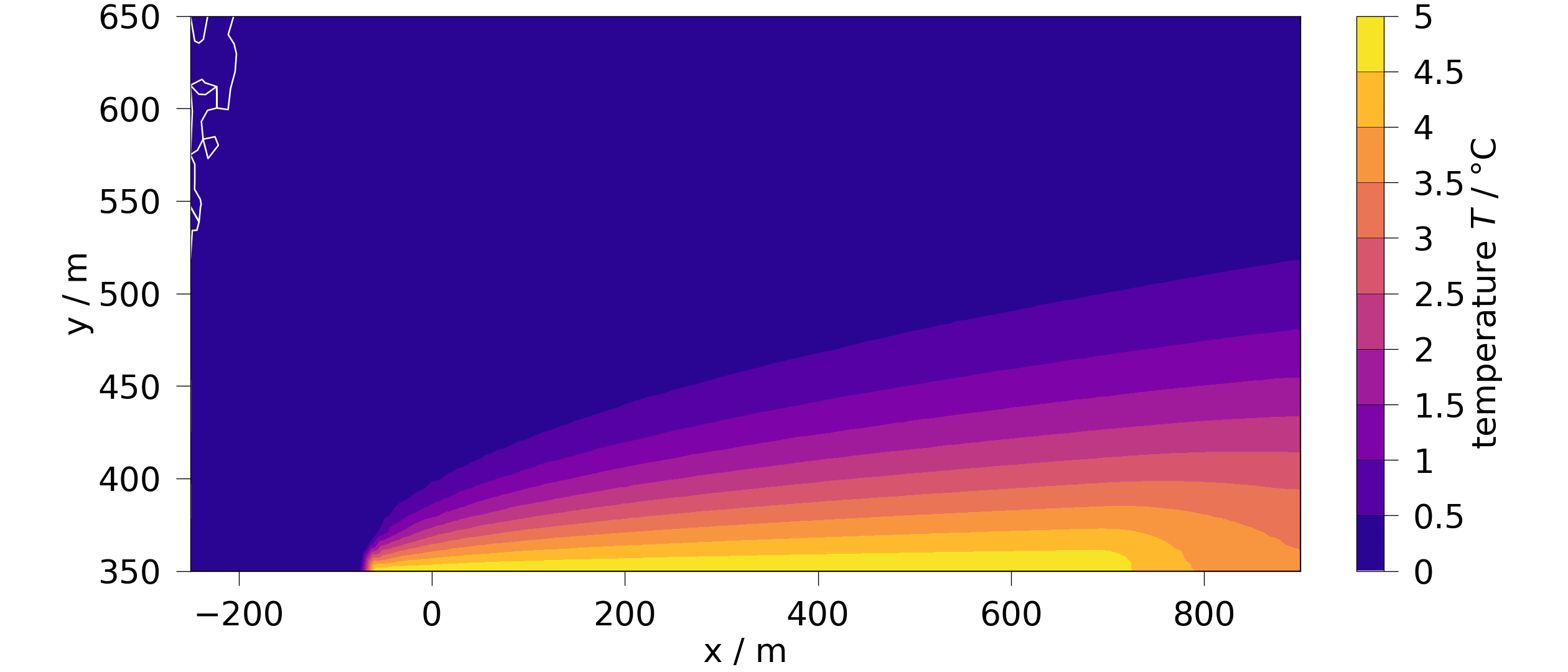
<Figure size 2520x1080 with 2 Axes>

6. The boundary meshes are manipulated to alter the model. The original boundary conditions are shown in this example: Workflow: Hydro-thermal model - conversion, simulation and post-processing 6.1 The Dirichlet boundary conditions for the hydraulic head are set to 0. Therefore, no water flows from the left to the right edge.

bc_flow = feflow_model.subdomains["P_BC_FLOW"]["P_BC_FLOW"]
feflow_model.subdomains["P_BC_FLOW"]["P_BC_FLOW"][bc_flow == 10] = 0

6.2 Overwrite the new boundary conditions and run the model.

feflow_model.run(overwrite=True)

OGS finished with project file /tmp/tmpeim6fyw1converted_models/HT_model.prj.
Execution took 1.4022948741912842 s
Project file written to output.

6.3 The corresponding simulation results look like.

ms = ot.MeshSeries(temp_dir / "HT_model.pvd")
# Read the last timestep:
ogs_sim_res = ms.mesh(ms.timesteps[-1])
ot.plot.contourf(ogs_sim_res, ot.variables.temperature)

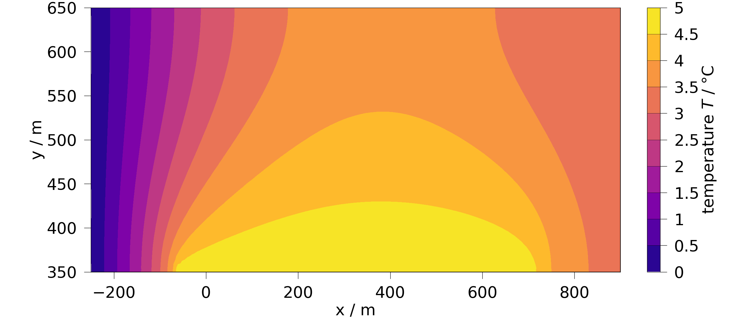
<Figure size 2520x1080 with 2 Axes>

6.4 Create a new boundary mesh and overwrite the existing subdomains with this boundary mesh.

assign_bulk_ids(mesh)
# Get the points of the bulk mesh to build a new boundary mesh.
wanted_pts = [1492, 1482, 1481, 1491, 1479, 1480, 1839, 1840]
new_bc = mesh.extract_points(
    [pt in wanted_pts for pt in mesh["bulk_node_ids"]],
    adjacent_cells=False,
    include_cells=False,
)
new_bc["bulk_node_ids"] = np.array(wanted_pts, dtype=np.uint64)
# Define the temperature values of these points.
new_bc["P_BC_HEAT"] = np.array([300] * len(wanted_pts), dtype=np.float64)
feflow_model.subdomains["P_BC_HEAT"] = new_bc

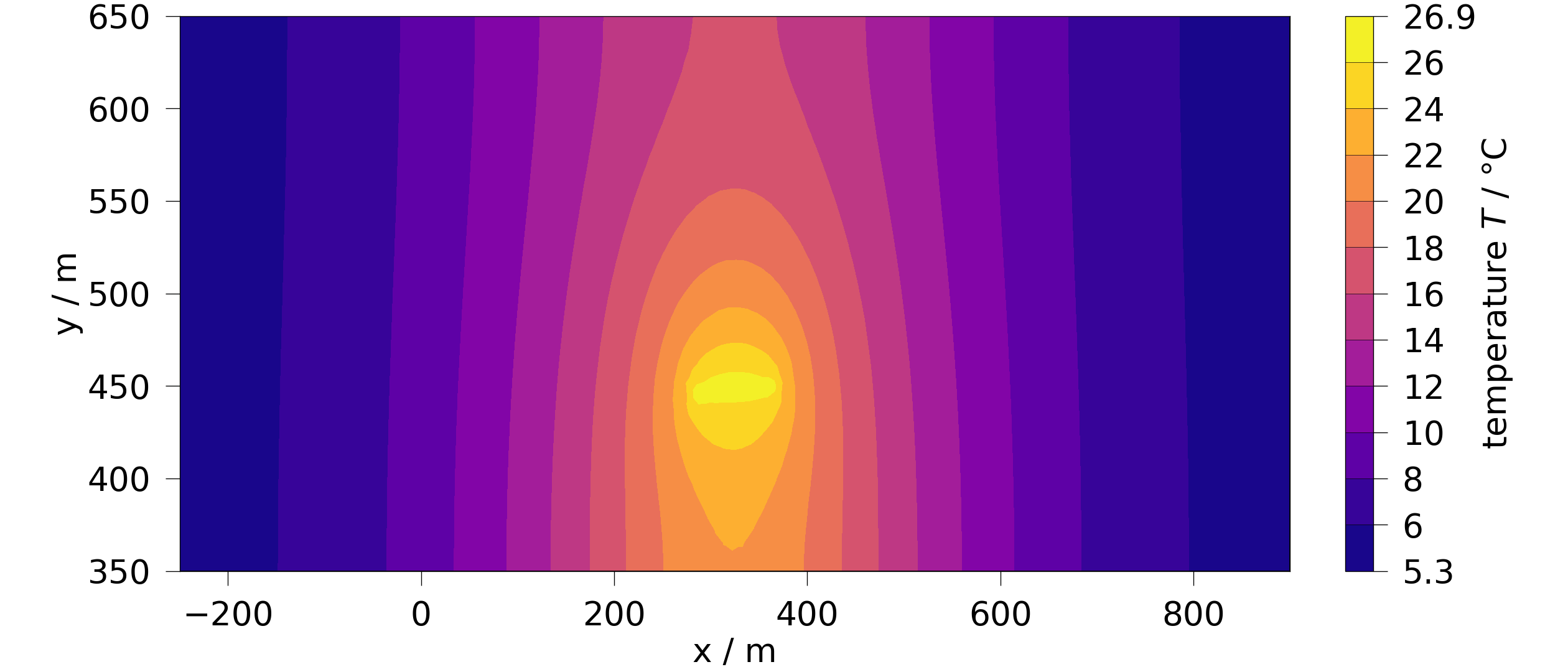
7. Run the new model and plot the simulation results.

feflow_model.run(overwrite=True)
ms = ot.MeshSeries(temp_dir / "HT_model.pvd")
ogs_sim_res = ms.mesh(ms.timesteps[-1])
ot.plot.contourf(ogs_sim_res, ot.variables.temperature)

OGS finished with project file /tmp/tmpeim6fyw1converted_models/HT_model.prj.
Execution took 1.419546365737915 s
Project file written to output.

<Figure size 2520x1080 with 2 Axes>