

Note
Go to the end to download the full example code.
Visualizing 2D model data#
Section author: Florian Zill (Helmholtz Centre for Environmental Research GmbH - UFZ)
To demonstrate the creation of filled contour plots we load a 2D THM meshseries
example. In the plot.setup we can provide a dictionary to map names
to material ids. Other plot configurations are also available, see:
ogstools.plot.plot_setup.PlotSetup. Some of these options are also
available as keyword arguments in the function call. Please see
ogstools.plot.contourplots.contourf for more information.
import ogstools as ot
from ogstools import examples

ot.plot.setup.material_names = {i + 1: f"Layer {i+1}" for i in range(26)}
mesh = examples.load_meshseries_THM_2D_PVD().scale(spatial=("m", "km")).mesh(1)
To read your own data as a mesh series you can do:
mesh_series = ot.MeshSeries("filepath/filename_pvd_or_xdmf")
the setup, this will automatically show the element edges.
fig = mesh.plot_contourf(ot.variables.material_id)
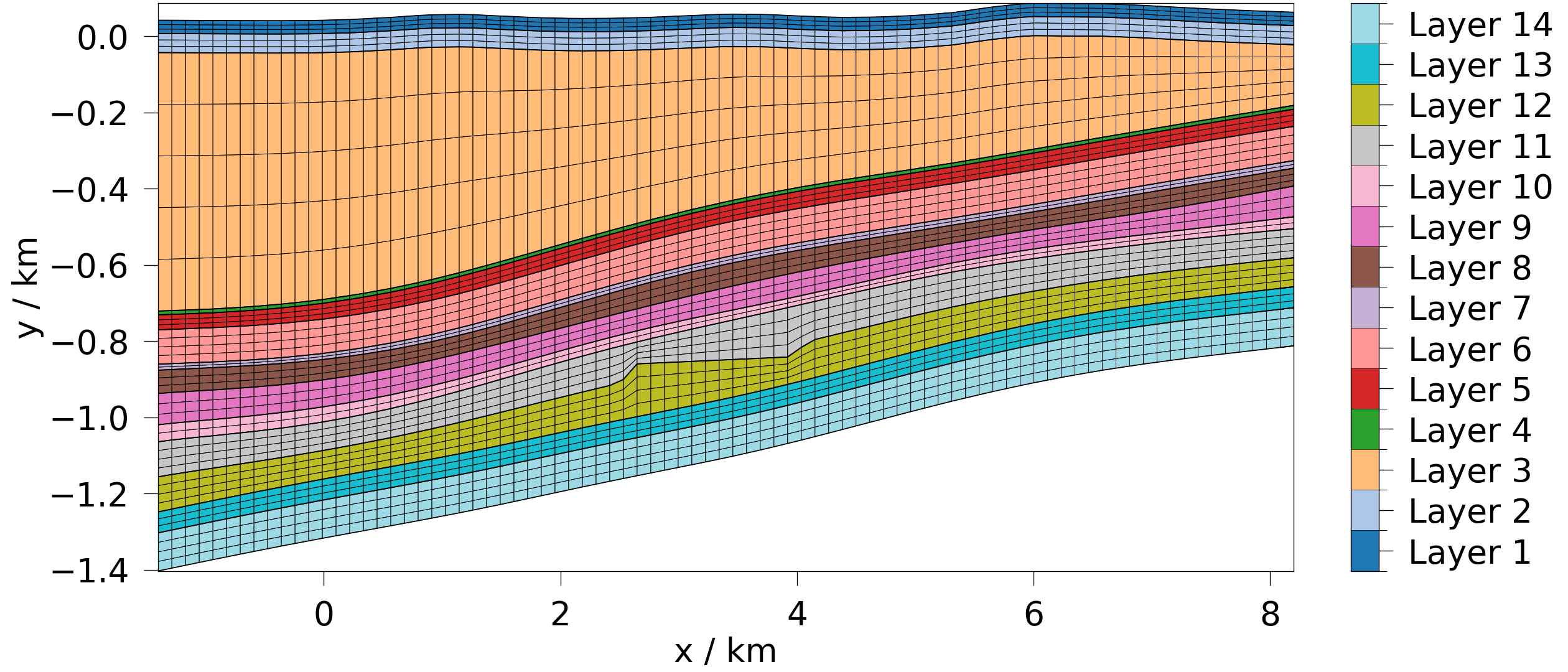
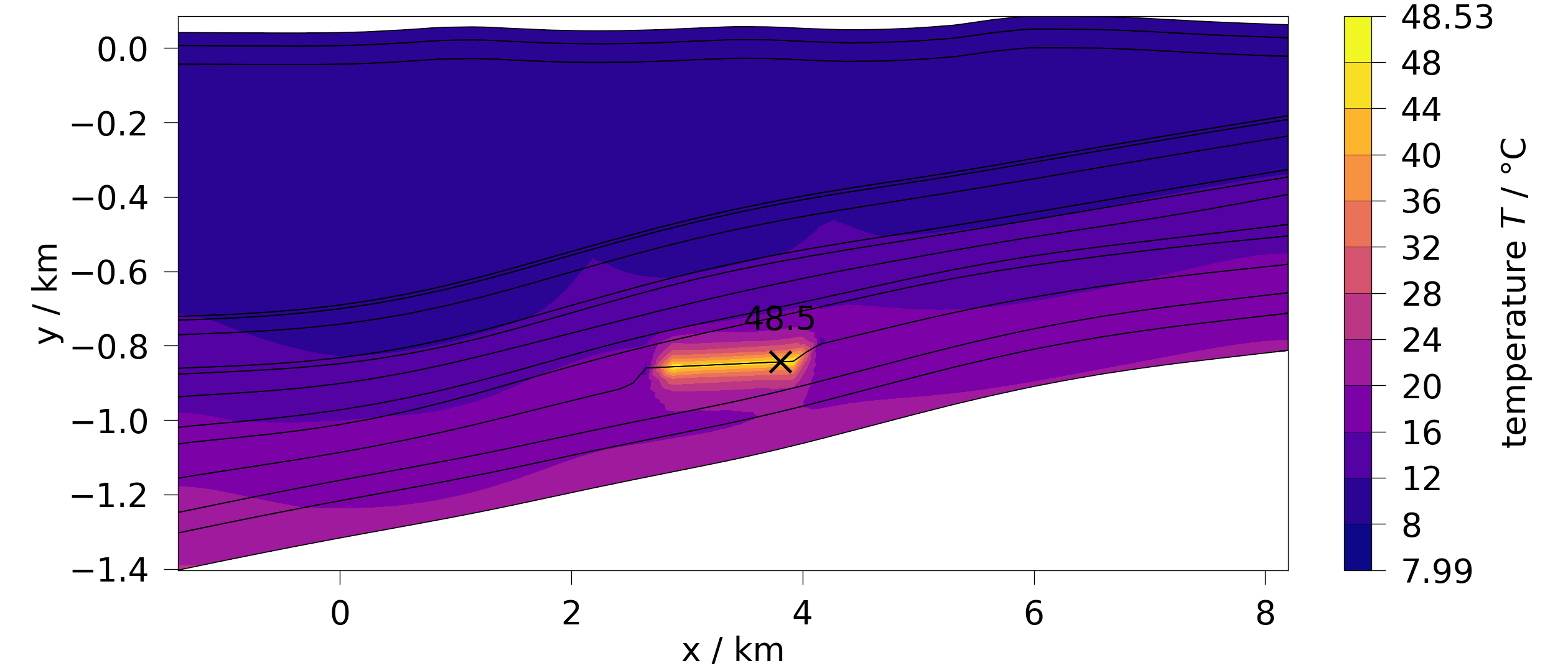
Now, let’s plot the temperature field (point_data) at the first timestep.
The default temperature variable from the variables reads the temperature
data as Kelvin and converts them to degrees Celsius.
fig = mesh.plot_contourf(ot.variables.temperature, show_max=True)
We can also plot components of vector variables:
fig = mesh.plot_contourf(
    ot.variables.displacement[0], show_min=True, show_max=True
)
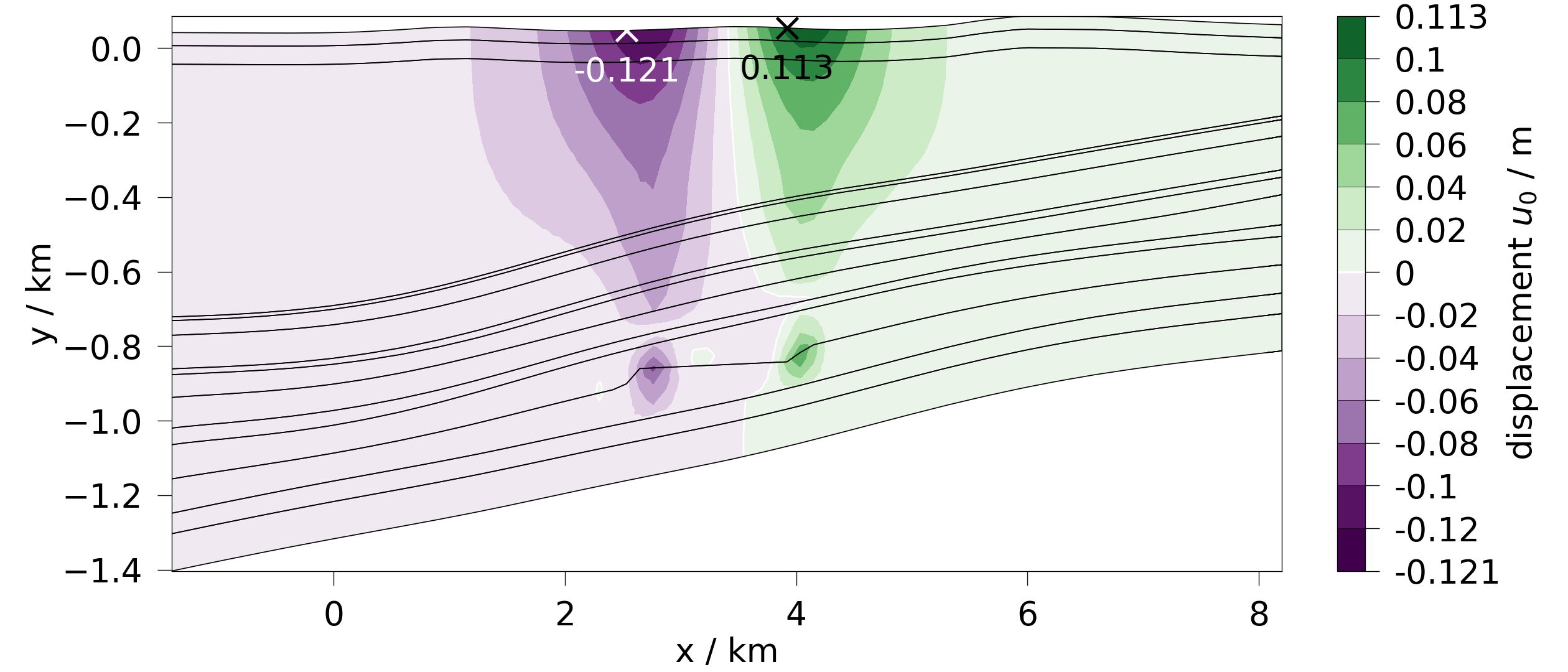
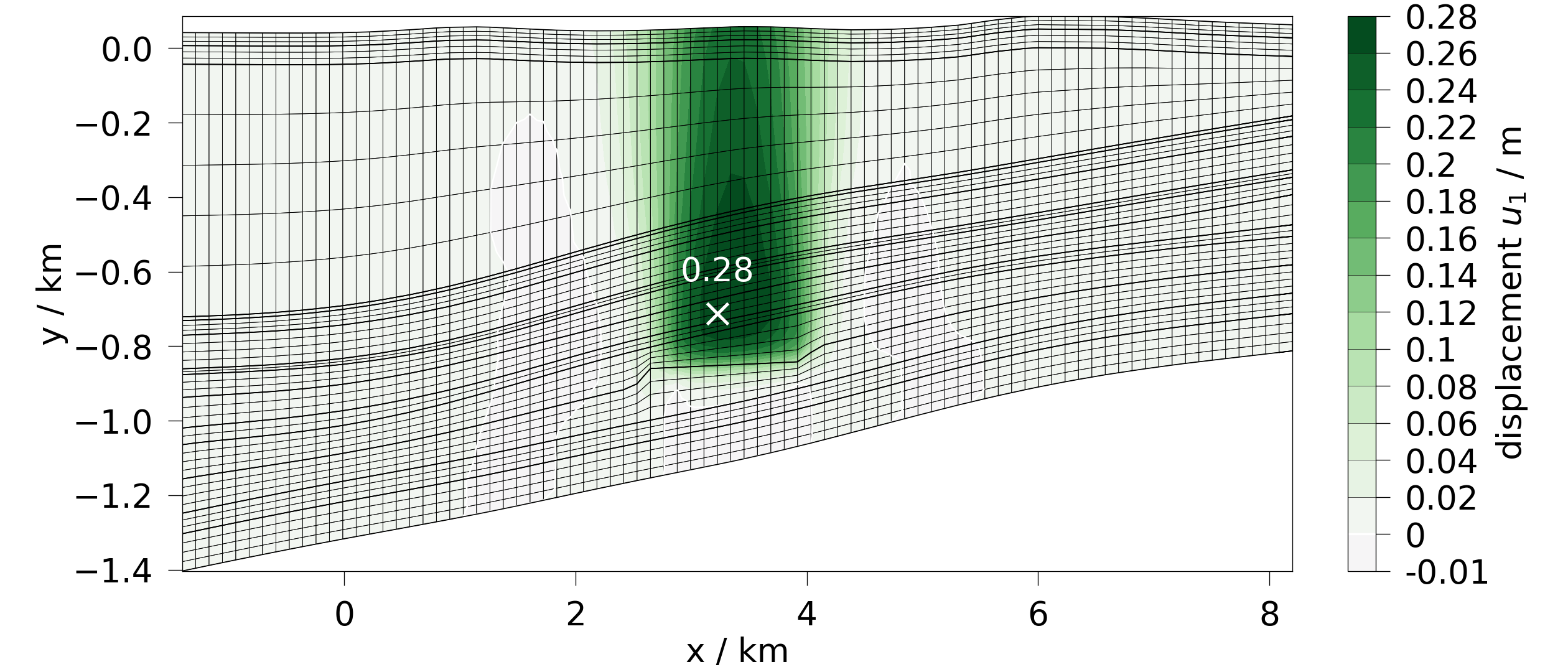
fig = mesh.plot_contourf(
    ot.variables.displacement[1], show_max=True, show_edges=True
)
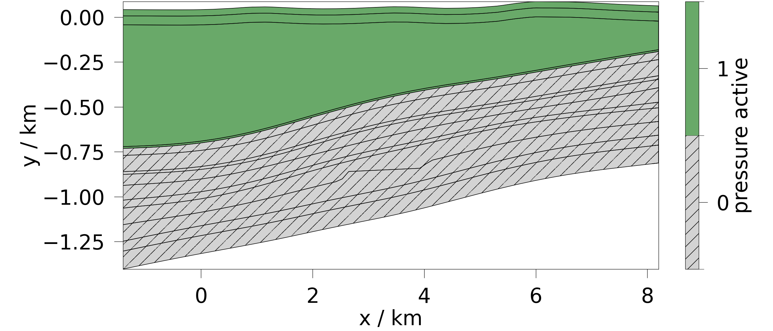
This example has hydraulically deactivated subdomains:
fig = mesh.plot_contourf(ot.variables.pressure.get_mask(), fontsize=40)
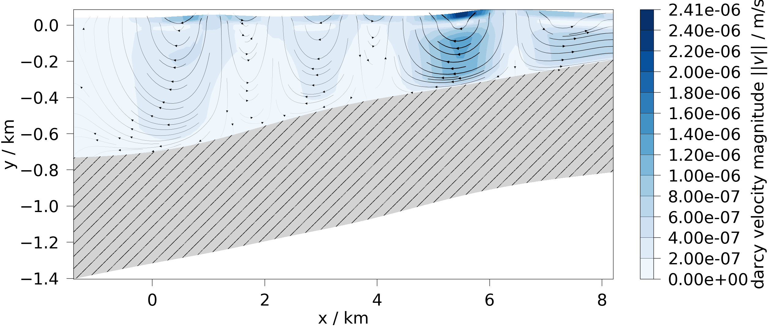
Let’s plot the fluid velocity field.
fig = mesh.plot_contourf(ot.variables.velocity, show_region_bounds=False)
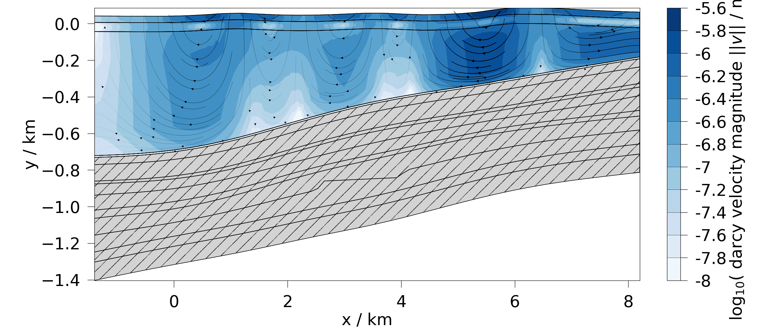
Let’s plot it again, this time log-scaled.
fig = mesh.plot_contourf(ot.variables.velocity, log_scaled=True, vmin=-8)
Total running time of the script: (0 minutes 5.185 seconds)