

Note
Go to the end to download the full example code or to run this example in your browser via Binder.
Workflow with Feflowlib: Component-transport model - conversion, simulation, postprocessing#
In this example we show how a simple mass transport FEFLOW model can be converted to a pyvista.UnstructuredGrid and then be simulated in OGS with the component transport process.
Necessary imports
import xml.etree.ElementTree as ET

import matplotlib.pyplot as plt

import ogstools as ot
from ogstools.examples import feflow_model_2D_CT_t_560

ot.plot.setup.show_element_edges = True
1. Load a FEFLOW model (.fem) as a FeflowModel object to further work it. During the initialisation, the FEFLOW file is converted.
temp_dir = ot.definitions.temp_dir("feflow_test_simulation", "examples")
feflow_model = ot.FeflowModel(
feflow_model_2D_CT_t_560, temp_dir / "2D_CT_model"
)
# name the feflow concentratiob result the same as in OGS for easier comparison
feflow_model.mesh["single_species"] = feflow_model.mesh["single_species_P_CONC"]
concentration = ot.variables.Scalar(
data_name="single_species", output_name="concentration",
data_unit="mg/l", output_unit="mg/l",
) # fmt: skip
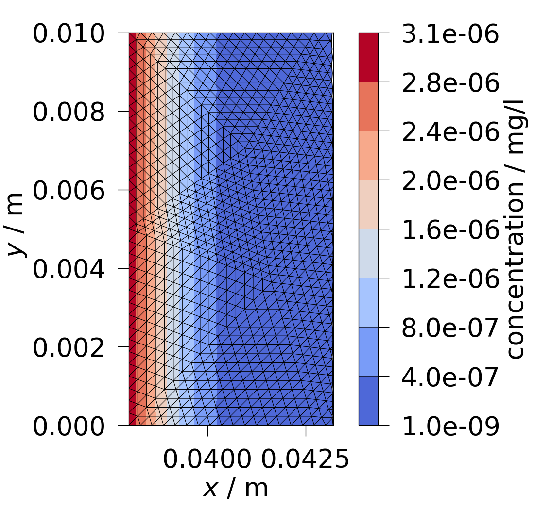
# The original mesh is clipped to focus on the relevant part of it, where
# concentration is larger than 1e-9 mg/l. The rest of the mesh has concentration
# values of 0.
clipped_mesh = feflow_model.mesh.clip_scalar(
scalars="single_species", invert=False, value=1.0e-9
)
ot.plot.contourf(clipped_mesh, concentration)
<Figure size 1099.71x1080 with 2 Axes>
Setup a prj-file to run a OGS-simulation.
time_steps = list(zip([10] * 8, [8.64 * 10**i for i in range(8)], strict=False))
feflow_model.setup_prj(end_time=int(4.8384e07), time_stepping=time_steps)
# Save the model (mesh, subdomains and project file).
feflow_model.save()
# Print the prj-file as an example.
ET.dump(ET.parse(feflow_model.mesh_path.with_suffix(".prj")))
<OpenGeoSysProject>
<meshes>
<mesh>2D_CT_model.vtu</mesh>
<mesh>single_species_P_BC_MASS.vtu</mesh>
</meshes>
<processes>
<process>
<name>CT</name>
<type>ComponentTransport</type>
<coupling_scheme>staggered</coupling_scheme>
<integration_order>2</integration_order>
<specific_body_force>0 0</specific_body_force>
<secondary_variables>
<secondary_variable internal_name="darcy_velocity" output_name="v" />
</secondary_variables>
<process_variables>
<pressure>HEAD_OGS</pressure>
<concentration>single_species</concentration>
</process_variables>
</process>
</processes>
<media>
<medium id="0">
<phases>
<phase>
<type>AqueousLiquid</type>
<properties>
<property>
<name>viscosity</name>
<type>Constant</type>
<value>1</value>
</property>
<property>
<name>density</name>
<type>Constant</type>
<value>1</value>
</property>
</properties>
<components>
<component>
<name>single_species</name>
<properties>
<property>
<name>decay_rate</name>
<type>Constant</type>
<value>0.0</value>
</property>
<property>
<name>pore_diffusion</name>
<type>Constant</type>
<value>3.5999998241701783e-10</value>
</property>
<property>
<name>retardation_factor</name>
<type>Constant</type>
<value>16441.72737282367</value>
</property>
</properties>
</component>
</components>
</phase>
</phases>
<properties>
<property>
<name>porosity</name>
<type>Constant</type>
<value>0.10999999940395355</value>
</property>
<property>
<name>longitudinal_dispersivity</name>
<type>Constant</type>
<value>0.0</value>
</property>
<property>
<name>transversal_dispersivity</name>
<type>Constant</type>
<value>0.0</value>
</property>
<property>
<name>permeability</name>
<type>Constant</type>
<value>1.1574074074074073e-05</value>
</property>
</properties>
</medium>
</media>
<time_loop>
<processes>
<process ref="CT">
<nonlinear_solver>basic_picard</nonlinear_solver>
<convergence_criterion>
<type>DeltaX</type>
<norm_type>NORM2</norm_type>
<reltol>1e-6</reltol>
</convergence_criterion>
<time_discretization>
<type>BackwardEuler</type>
</time_discretization>
<time_stepping>
<type>FixedTimeStepping</type>
<t_initial>0</t_initial>
<t_end>48384000</t_end>
<timesteps>
<pair>
<repeat>10</repeat>
<delta_t>8.64</delta_t>
</pair>
<pair>
<repeat>10</repeat>
<delta_t>86.4</delta_t>
</pair>
<pair>
<repeat>10</repeat>
<delta_t>864.0</delta_t>
</pair>
<pair>
<repeat>10</repeat>
<delta_t>8640.0</delta_t>
</pair>
<pair>
<repeat>10</repeat>
<delta_t>86400.0</delta_t>
</pair>
<pair>
<repeat>10</repeat>
<delta_t>864000.0</delta_t>
</pair>
<pair>
<repeat>10</repeat>
<delta_t>8640000.0</delta_t>
</pair>
<pair>
<repeat>10</repeat>
<delta_t>86400000.0</delta_t>
</pair>
</timesteps>
</time_stepping>
</process>
</processes>
<output>
<type>VTK</type>
<prefix>/tmp/ogstools_root/examples/feflow_test_simulationee3834e952b64e67aba68b2b5ef0d2b9/2D_CT_model</prefix>
<timesteps>
<pair>
<repeat>1</repeat>
<each_steps>1</each_steps>
</pair>
</timesteps>
<variables>
<variable>single_species</variable>
<variable>HEAD_OGS</variable>
</variables>
<fixed_output_times>48384000</fixed_output_times>
</output>
<global_process_coupling>
<max_iter>1</max_iter>
<convergence_criteria>
<convergence_criterion>
<type>DeltaX</type>
<norm_type>NORM2</norm_type>
<reltol>1e-10</reltol>
</convergence_criterion>
<convergence_criterion>
<type>DeltaX</type>
<norm_type>NORM2</norm_type>
<reltol>1e-10</reltol>
</convergence_criterion>
</convergence_criteria>
</global_process_coupling>
</time_loop>
<parameters>
<parameter>
<name>C0</name>
<type>Constant</type>
<value>0</value>
</parameter>
<parameter>
<name>p0</name>
<type>Constant</type>
<value>0</value>
</parameter>
<parameter>
<name>single_species_P_BC_MASS</name>
<type>MeshNode</type>
<mesh>single_species_P_BC_MASS</mesh>
<field_name>single_species_P_BC_MASS</field_name>
</parameter>
</parameters>
<process_variables>
<process_variable>
<name>single_species</name>
<components>1</components>
<order>1</order>
<initial_condition>C0</initial_condition>
<boundary_conditions>
<boundary_condition>
<type>Dirichlet</type>
<mesh>single_species_P_BC_MASS</mesh>
<parameter>single_species_P_BC_MASS</parameter>
</boundary_condition>
</boundary_conditions>
</process_variable>
<process_variable>
<name>HEAD_OGS</name>
<components>1</components>
<order>1</order>
<initial_condition>p0</initial_condition>
</process_variable>
</process_variables>
<nonlinear_solvers>
<nonlinear_solver>
<name>basic_picard</name>
<type>Picard</type>
<max_iter>100</max_iter>
<linear_solver>general_linear_solver</linear_solver>
</nonlinear_solver>
</nonlinear_solvers>
<linear_solvers>
<linear_solver>
<name>general_linear_solver</name>
<lis>-i cg -p jacobi -tol 1e-10 -maxiter 100000</lis>
<eigen>
<solver_type>CG</solver_type>
<precon_type>DIAGONAL</precon_type>
<max_iteration_step>100000</max_iteration_step>
<error_tolerance>1e-10</error_tolerance>
</eigen>
</linear_solver>
</linear_solvers>
</OpenGeoSysProject>
Run the model.
feflow_model.run()
 ogs  -o . /tmp/ogstools_root/examples/feflow_test_simulationee3834e952b64e67aba68b2b5ef0d2b9/2D_CT_model.prj
['ogs', '-o', '.', '/tmp/ogstools_root/examples/feflow_test_simulationee3834e952b64e67aba68b2b5ef0d2b9/2D_CT_model.prj']
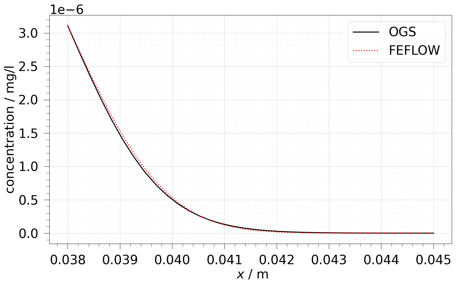
4. Read the last timestep and plot the results along a line on the upper edge of the mesh parallel to the x-axis.
ogs_sim_res = ot.MeshSeries(temp_dir / "2D_CT_model.pvd")[-1]
fig, ax = plt.subplots(1, 1, figsize=(16, 10))
pts = [[0.038 + 1.0e-8, 0.005, 0], [0.045, 0.005, 0]]
for i, mesh in enumerate([ogs_sim_res, feflow_model.mesh]):
    sample = mesh.sample_over_line(*pts)
    label = ["OGS", "FEFLOW"][i]
    ot.plot.line(
        sample, concentration, ax=ax, color="kr"[i], label=label, ls="-:"[i]
    )
fig.tight_layout()
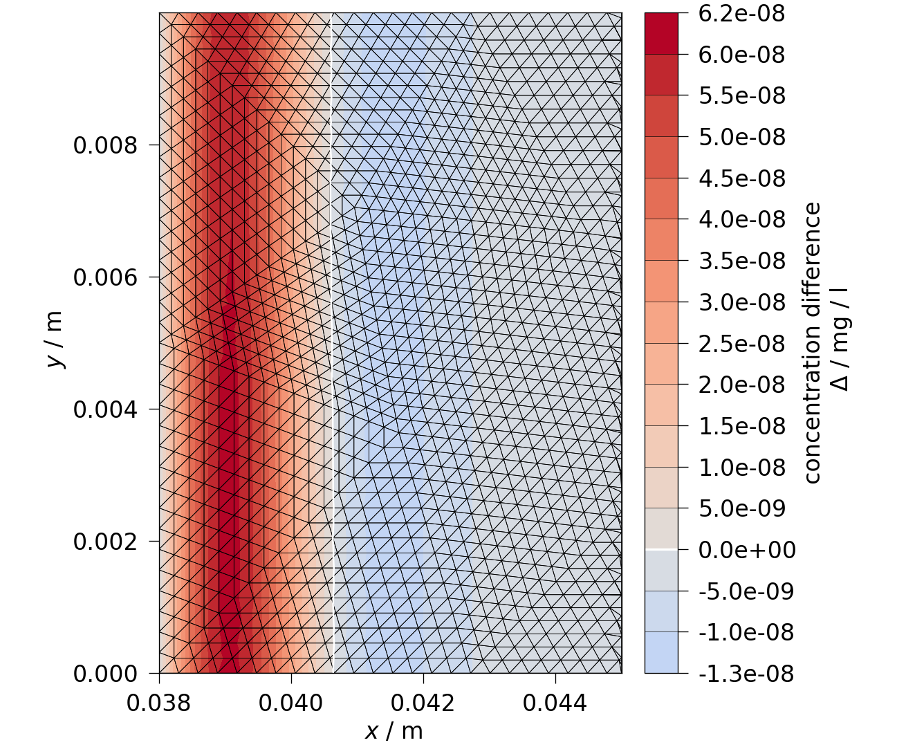
Concentration difference plotted on the mesh.
diff = ot.mesh.difference(feflow_model.mesh, ogs_sim_res, concentration)
diff_clipped = diff.clip_box([0.038, 0.045, 0, 0.01, 0, 0], invert=False)
fig = ot.plot.contourf(diff_clipped, concentration.difference, fontsize=20)
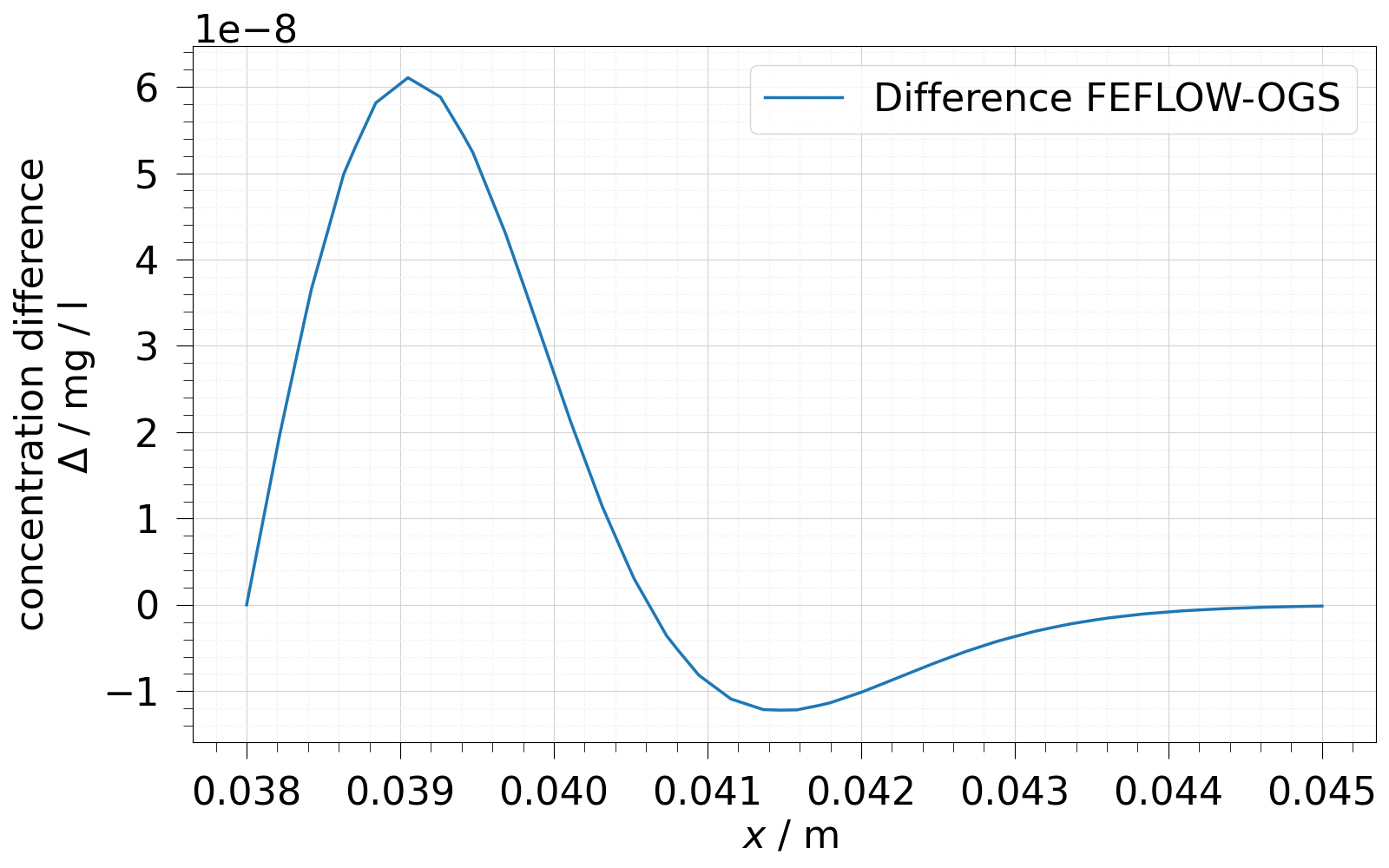
5.1 Concentration difference plotted along a line.
diff_sample = diff.sample_over_line(*pts)
fig = ot.plot.line(
    diff_sample, concentration.difference, label="Difference FEFLOW-OGS"
)
fig.tight_layout()
Total running time of the script: (0 minutes 4.072 seconds)