Note
Go to the end to download the full example code.
Feflowlib: Hydro-thermal model - conversion and simulation#
Section author: Julian Heinze (Helmholtz Centre for Environmental Research GmbH - UFZ)
In this example we show how a simple hydro thermal FEFLOW model can be converted to a pyvista.UnstructuredGrid and then be simulated in OGS.
Necessary imports
import tempfile
import xml.etree.ElementTree as ET
from pathlib import Path
import ifm_contrib as ifm
import pyvista as pv
import ogstools as ogs
from ogstools.examples import feflow_model_2D_HT_model
from ogstools.feflowlib import (
convert_properties_mesh,
hydro_thermal,
setup_prj_file,
)
from ogstools.feflowlib.tools import (
extract_point_boundary_conditions,
get_material_properties_of_HT_model,
)
1. Load a FEFLOW model (.fem) as a FEFLOW document, convert and save it. More details on
how the conversion function works can be found here: ogstools.feflowlib.convert_properties_mesh
.
feflow_model = ifm.loadDocument(str(feflow_model_2D_HT_model))
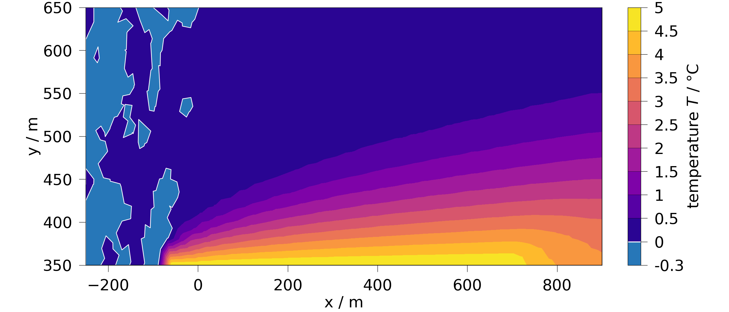
feflow_pv_mesh = convert_properties_mesh(feflow_model)
feflow_temperature = ogs.variables.temperature.replace(data_name="P_TEMP")
ogs.plot.contourf(feflow_pv_mesh, feflow_temperature)
temp_dir = Path(tempfile.mkdtemp("feflow_test_simulation"))
feflow_mesh_file = temp_dir / "2D_HT_model.vtu"
feflow_pv_mesh.save(feflow_mesh_file)
print(feflow_pv_mesh)
UnstructuredGrid (0x7cd46b5849a0)
N Cells: 1565
N Points: 832
X Bounds: -2.500e+02, 9.000e+02
Y Bounds: 3.500e+02, 6.500e+02
Z Bounds: 0.000e+00, 0.000e+00
N Arrays: 34
Extract the point conditions (see:
ogstools.feflowlib.extract_point_boundary_conditions
).
point_BC_dict = extract_point_boundary_conditions(temp_dir, feflow_pv_mesh)
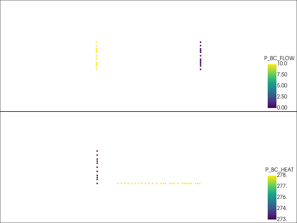
# Since there can be multiple point boundary conditions on the bulk mesh, they are plotted iteratively.
plotter = pv.Plotter(shape=(len(point_BC_dict), 1))
for i, (path, boundary_condition) in enumerate(point_BC_dict.items()):
boundary_condition.save(path)
plotter.subplot(i, 0)
plotter.add_mesh(boundary_condition, scalars=Path(path).stem)
plotter.view_xy()
plotter.show()
Setup a prj-file (see:
ogstools.feflowlib.setup_prj_file
) to run a OGS-simulation.
path_prjfile = feflow_mesh_file.with_suffix(".prj")
prj = ogs.Project(output_file=path_prjfile)
# Get the template prj-file configurations for a hydro thermal process.
HT_model = hydro_thermal(temp_dir / "sim_2D_HT_model", prj, dimension=2)
# Include the mesh specific configurations to the template.
model = setup_prj_file(
bulk_mesh_path=feflow_mesh_file,
mesh=feflow_pv_mesh,
material_properties=get_material_properties_of_HT_model(feflow_pv_mesh),
process="hydro thermal",
model=HT_model,
)
# The model must be written before it can be run.
model.write_input(path_prjfile)
# Print the prj-file as an example.
model_prjfile = ET.parse(path_prjfile)
ET.dump(model_prjfile)
<OpenGeoSysProject>
<meshes>
<mesh>2D_HT_model.vtu</mesh>
<mesh>P_BC_FLOW.vtu</mesh>
<mesh>P_BC_HEAT.vtu</mesh>
</meshes>
<processes>
<process>
<name>HydroThermal</name>
<type>HT</type>
<integration_order>3</integration_order>
<specific_body_force>0 0</specific_body_force>
<secondary_variables>
<secondary_variable internal_name="darcy_velocity" output_name="v" />
</secondary_variables>
<process_variables>
<temperature>temperature</temperature>
<pressure>HEAD_OGS</pressure>
</process_variables>
</process>
</processes>
<media>
<medium id="0">
<phases>
<phase>
<type>AqueousLiquid</type>
<properties>
<property>
<name>specific_heat_capacity</name>
<type>Constant</type>
<value>4200000.0</value>
</property>
<property>
<name>thermal_conductivity</name>
<type>Constant</type>
<value>0.65</value>
</property>
<property>
<name>viscosity</name>
<type>Constant</type>
<value>1</value>
</property>
<property>
<name>density</name>
<type>Constant</type>
<value>1</value>
</property>
</properties>
</phase>
<phase>
<type>Solid</type>
<properties>
<property>
<name>storage</name>
<type>Constant</type>
<value>0.0</value>
</property>
<property>
<name>density</name>
<type>Constant</type>
<value>1</value>
</property>
<property>
<name>specific_heat_capacity</name>
<type>Constant</type>
<value>1633000.0</value>
</property>
<property>
<name>thermal_conductivity</name>
<type>Constant</type>
<value>3.0</value>
</property>
</properties>
</phase>
</phases>
<properties>
<property>
<name>permeability</name>
<type>Constant</type>
<value>1.1574074074074073e-05 1.1574074074074073e-05</value>
</property>
<property>
<name>porosity</name>
<type>Constant</type>
<value>0.0</value>
</property>
<property>
<name>thermal_conductivity</name>
<type>EffectiveThermalConductivityPorosityMixing</type>
</property>
<property>
<name>thermal_transversal_dispersivity</name>
<type>Constant</type>
<value>0.5</value>
</property>
<property>
<name>thermal_longitudinal_dispersivity</name>
<type>Constant</type>
<value>5.0</value>
</property>
</properties>
</medium>
</media>
<time_loop>
<processes>
<process ref="HydroThermal">
<nonlinear_solver>basic_picard</nonlinear_solver>
<convergence_criterion>
<type>DeltaX</type>
<norm_type>NORM2</norm_type>
<abstol>1e-16</abstol>
</convergence_criterion>
<time_discretization>
<type>BackwardEuler</type>
</time_discretization>
<time_stepping>
<type>FixedTimeStepping</type>
<t_initial>0</t_initial>
<t_end>1e11</t_end>
<timesteps>
<pair>
<repeat>1</repeat>
<delta_t>1e10</delta_t>
</pair>
<pair>
<repeat>1</repeat>
<delta_t>1e10</delta_t>
</pair>
</timesteps>
</time_stepping>
</process>
</processes>
<output>
<type>VTK</type>
<prefix>/tmp/tmpclvdkfizfeflow_test_simulation/sim_2D_HT_model</prefix>
<timesteps>
<pair>
<repeat>1</repeat>
<each_steps>1</each_steps>
</pair>
</timesteps>
<variables />
</output>
</time_loop>
<parameters>
<parameter>
<name>T0</name>
<type>Constant</type>
<value>273.15</value>
</parameter>
<parameter>
<name>p0</name>
<type>Constant</type>
<value>0</value>
</parameter>
<parameter>
<name>P_BC_FLOW</name>
<type>MeshNode</type>
<mesh>P_BC_FLOW</mesh>
<field_name>P_BC_FLOW</field_name>
</parameter>
<parameter>
<name>P_BC_HEAT</name>
<type>MeshNode</type>
<mesh>P_BC_HEAT</mesh>
<field_name>P_BC_HEAT</field_name>
</parameter>
</parameters>
<process_variables>
<process_variable>
<name>temperature</name>
<components>1</components>
<order>1</order>
<initial_condition>T0</initial_condition>
<boundary_conditions>
<boundary_condition>
<type>Dirichlet</type>
<mesh>P_BC_HEAT</mesh>
<parameter>P_BC_HEAT</parameter>
</boundary_condition>
</boundary_conditions>
</process_variable>
<process_variable>
<name>HEAD_OGS</name>
<components>1</components>
<order>1</order>
<initial_condition>p0</initial_condition>
<boundary_conditions>
<boundary_condition>
<type>Dirichlet</type>
<mesh>P_BC_FLOW</mesh>
<parameter>P_BC_FLOW</parameter>
</boundary_condition>
</boundary_conditions>
</process_variable>
</process_variables>
<nonlinear_solvers>
<nonlinear_solver>
<name>basic_picard</name>
<type>Picard</type>
<max_iter>100</max_iter>
<linear_solver>general_linear_solver</linear_solver>
</nonlinear_solver>
</nonlinear_solvers>
<linear_solvers>
<linear_solver>
<name>general_linear_solver</name>
<lis>-i bicgstab -p jacobi -tol 1e-20 -maxiter 10000</lis>
<eigen>
<solver_type>SparseLU</solver_type>
<scaling>true</scaling>
</eigen>
</linear_solver>
</linear_solvers>
</OpenGeoSysProject>
Run the model.
model.run_model(logfile=temp_dir / "out.log")
OGS finished with project file /tmp/tmpclvdkfizfeflow_test_simulation/2D_HT_model.prj.
Execution took 0.4532768726348877 s
Project file written to output.
Read the results and plot them.
ms = ogs.MeshSeries(temp_dir / "sim_2D_HT_model.pvd")
# Read the last timestep:
ogs_sim_res = ms.mesh(ms.timesteps[-1])
"""
It is also possible to read the file directly with pyvista:
ogs_sim_res = pv.read(
temp_dir / "sim_2D_HT_model_ts_10_t_100000000000.000000.vtu"
)
"""
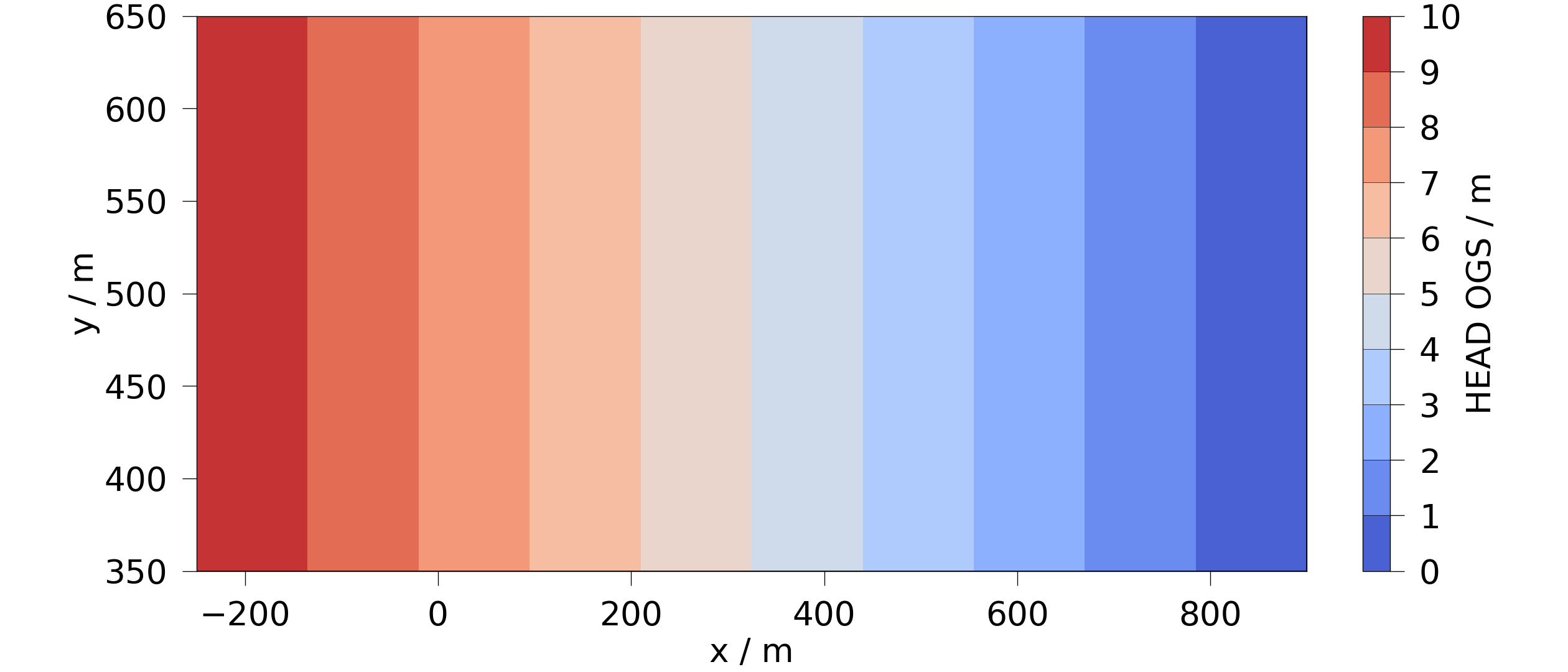
# Plot the hydraulic head/height, which was simulated in OGS.
hydraulic_head = ogs.variables.Scalar(
data_name="HEAD_OGS", data_unit="m", output_unit="m"
)
ogs.plot.contourf(ogs_sim_res, hydraulic_head)
<Figure size 2520x1080 with 2 Axes>
Plot the temperature, which was simulated in OGS.
ogs.plot.contourf(ogs_sim_res, ogs.variables.temperature)
<Figure size 2520x1080 with 2 Axes>
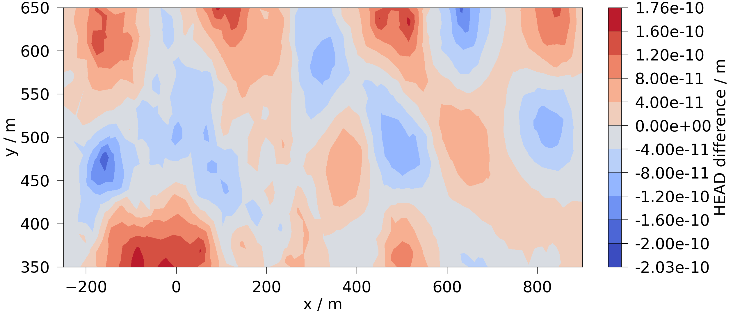
Plot the difference between the FEFLOW and OGS simulation.
feflow_pv_mesh["HEAD"] = feflow_pv_mesh["P_HEAD"]
ogs_sim_res["HEAD"] = ogs_sim_res["HEAD_OGS"]
# Plot differences in hydraulic head/height.
diff_mesh = ogs.meshlib.difference(feflow_pv_mesh, ogs_sim_res, "HEAD")
hydraulic_head_diff = ogs.variables.Scalar(
data_name="HEAD_difference", data_unit="m", output_unit="m"
)
ogs.plot.contourf(diff_mesh, hydraulic_head_diff)
<Figure size 2520x1080 with 2 Axes>
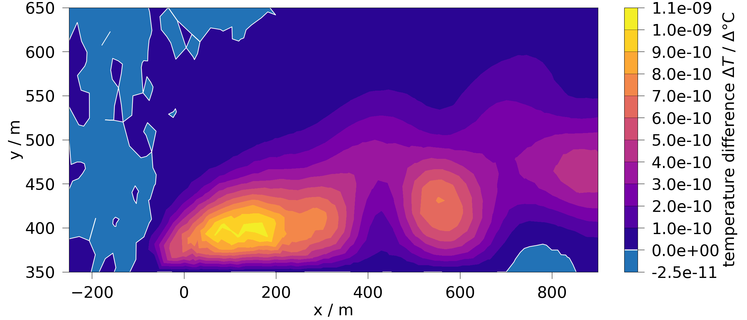
feflow_pv_mesh["temperature"] = feflow_pv_mesh["P_TEMP"]
# Plot differences in temperature.
diff_mesh = ogs.meshlib.difference(
feflow_pv_mesh, ogs_sim_res, ogs.variables.temperature
)
ogs.plot.contourf(diff_mesh, ogs.variables.temperature.difference)
<Figure size 2520x1080 with 2 Axes>
Total running time of the script: (0 minutes 2.018 seconds)