Workflow: Hydraulic model - conversion, simulation and post-processing

Section author: Julian Heinze (Helmholtz Centre for Environmental Research GmbH - UFZ)

In this example we show how a simple flow/hydraulic FEFLOW model can be converted to a pyvista.UnstructuredGrid and then be simulated in ot.

0. Necessary imports

import tempfile
from pathlib import Path

import numpy as np
import pyvista as pv

import ogstools as ot
from ogstools.examples import feflow_model_box_Neumann
from ogstools.feflowlib import (
    FeflowModel,
)

1. Load a FEFLOW model (.fem) as a FeflowModel object to further work it. During the initialisation, the FEFLOW file is converted.

temp_dir = Path(tempfile.mkdtemp("feflow_test_simulation"))
feflow_model = FeflowModel(feflow_model_box_Neumann, temp_dir / "boxNeumann")
pv.global_theme.colorbar_orientation = "vertical"
feflow_model.mesh.plot(
    show_edges=True,
    off_screen=True,
    scalars="P_HEAD",
    cpos=[0, 1, 0.5],
    scalar_bar_args={"position_x": 0.1, "position_y": 0.25},
)
print(feflow_model.mesh)

Static Scene

Interactive Scene

UnstructuredGrid (0x7b26fffe23e0)
  N Cells:    11462
  N Points:   6768
  X Bounds:   0.000e+00, 1.000e+02
  Y Bounds:   0.000e+00, 1.000e+02
  Z Bounds:   -1.000e+02, 0.000e+00
  N Arrays:   23

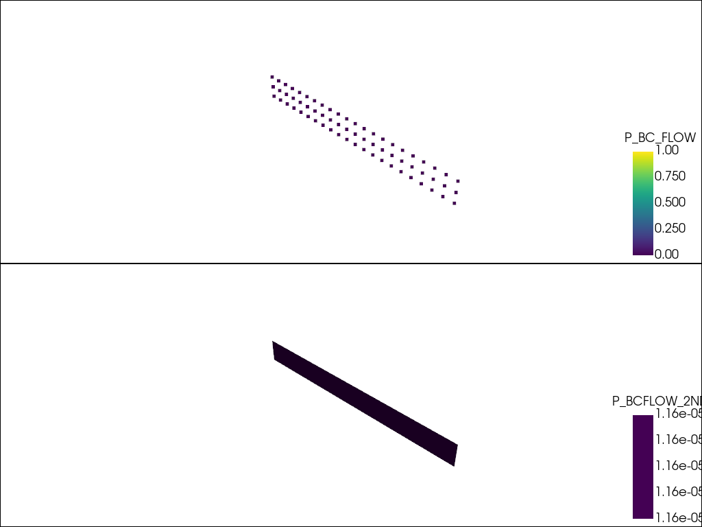
2. Extract the subdomains conditions.

subdomains = feflow_model.subdomains
# Since there can be multiple boundary conditions in the subdomains,
# they are plotted iteratively.
plotter = pv.Plotter(shape=(len(subdomains), 1))
for i, (name, boundary_condition) in enumerate(subdomains.items()):
    # topsurface refers to a cell based boundary condition.
    if name != "topsurface":
        plotter.subplot(i, 0)
        plotter.add_mesh(boundary_condition, scalars=name)
plotter.show()

Static Scene

Interactive Scene

3. Define endtime and time stepping in the project-file.

feflow_model.setup_prj(
    end_time=int(1e8),
    time_stepping=[(1, 10), (5, 100), (10, 1000), (10, 1e6), (1, 1e7)],
)

4. Run the model

feflow_model.run()

OGS finished with project file /tmp/tmppbvw3lwpfeflow_test_simulation/boxNeumann.prj.
Execution took 2.545957326889038 s
Project file written to output.

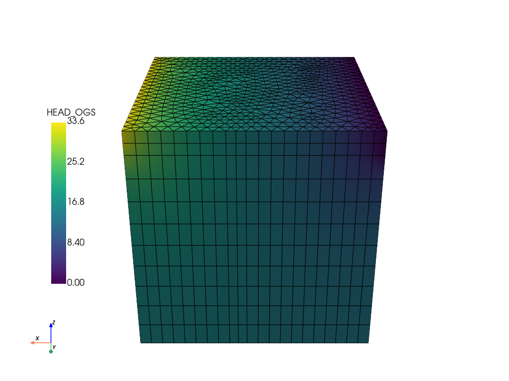
5. Read the results and plot them.

ms = ot.MeshSeries(temp_dir / "boxNeumann.pvd")
# Read the last timestep:
ogs_sim_res = ms.mesh(ms.timesteps[-1])
"""
It is also possible to read the file directly with pyvista:
ogs_sim_res = pv.read(temp_dir / "boxNeumann_ts_1_t_1.000000.vtu")
"""
ogs_sim_res.plot(
    show_edges=True,
    off_screen=True,
    scalars="HEAD_OGS",
    cpos=[0, 1, 0.5],
    scalar_bar_args={"position_x": 0.1, "position_y": 0.25},
)

Static Scene

Interactive Scene

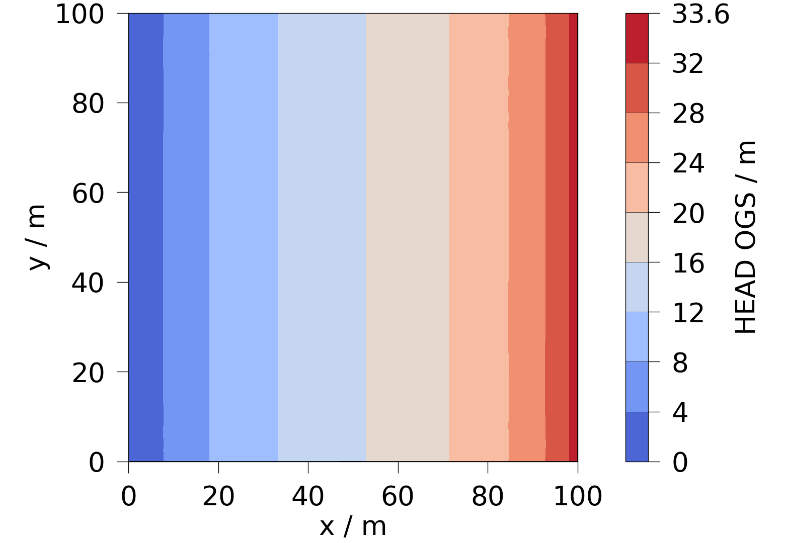
5.1 Plot the hydraulic head simulated in OGS with ogstools.plot.contourf.

head = ot.variables.Scalar(data_name="HEAD_OGS", data_unit="m", output_unit="m")
fig = ot.plot.contourf(ogs_sim_res.slice(normal="z", origin=[50, 50, 0]), head)

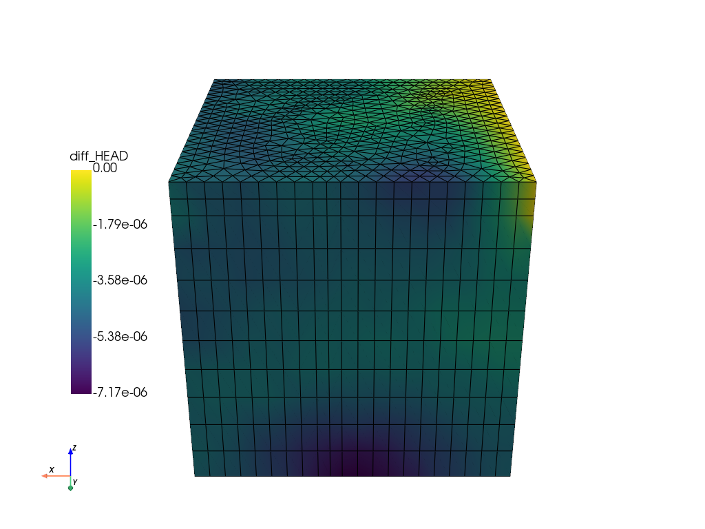
6. Calculate the difference to the FEFLOW simulation and plot it.

diff = feflow_model.mesh["P_HEAD"] - ogs_sim_res["HEAD_OGS"]
feflow_model.mesh["diff_HEAD"] = diff
feflow_model.mesh.plot(
    show_edges=True,
    off_screen=True,
    scalars="diff_HEAD",
    cpos=[0, 1, 0.5],
    scalar_bar_args={"position_x": 0.1, "position_y": 0.25},
)

Static Scene

Interactive Scene

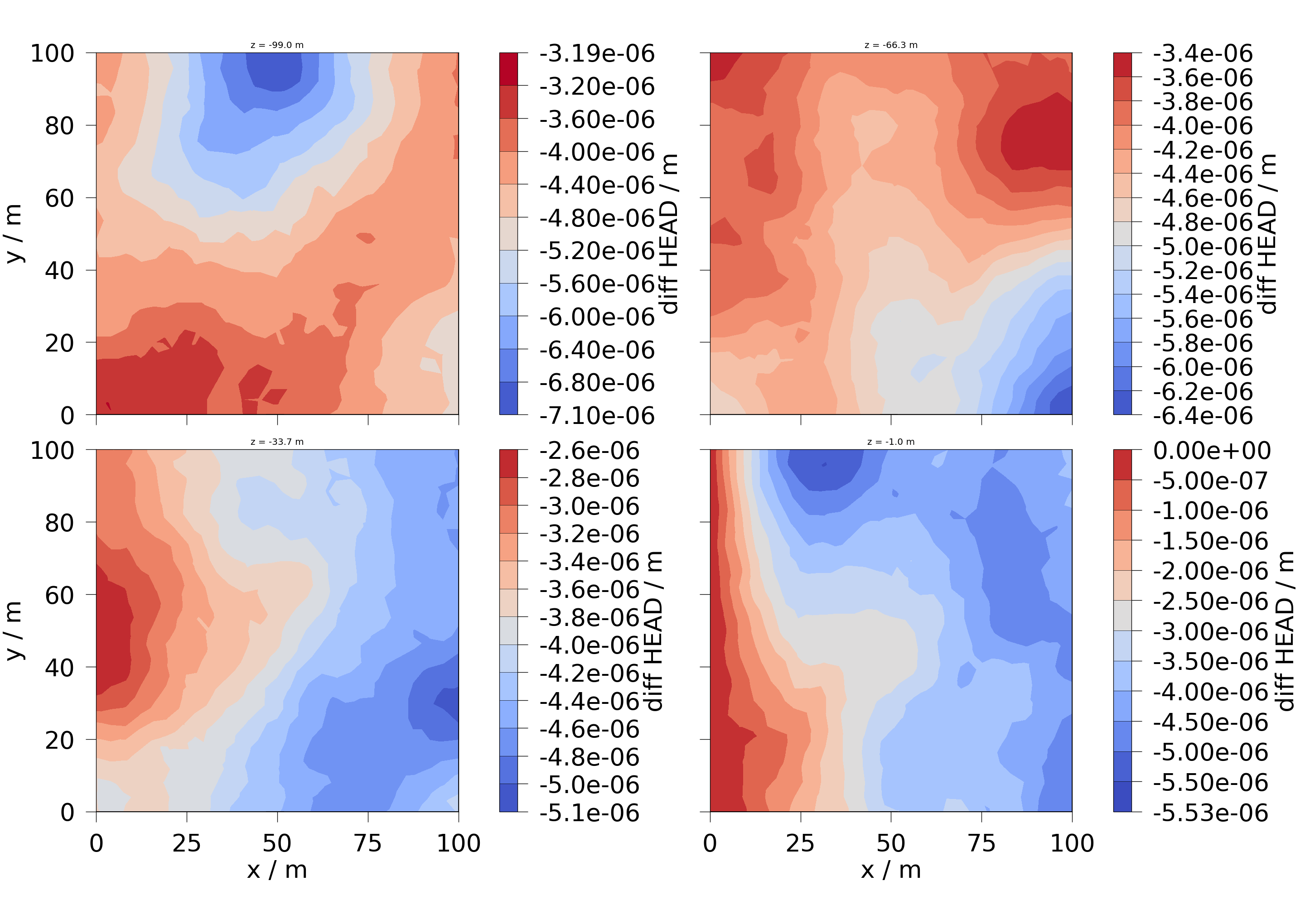
6.1 Plot the differences in the hydraulic head with ogstools.plot.contourf. Slices are taken along the z-axis.

diff_head = ot.variables.Scalar(
    data_name="diff_HEAD", data_unit="m", output_unit="m"
)
slices = np.reshape(
    list(feflow_model.mesh.slice_along_axis(n=4, axis="z")), (2, 2)
)
fig = ot.plot.contourf(slices, diff_head)
for ax, slice in zip(fig.axes, np.ravel(slices), strict=False):
    ax.set_title(f"z = {slice.center[2]:.1f} m", fontsize=32)

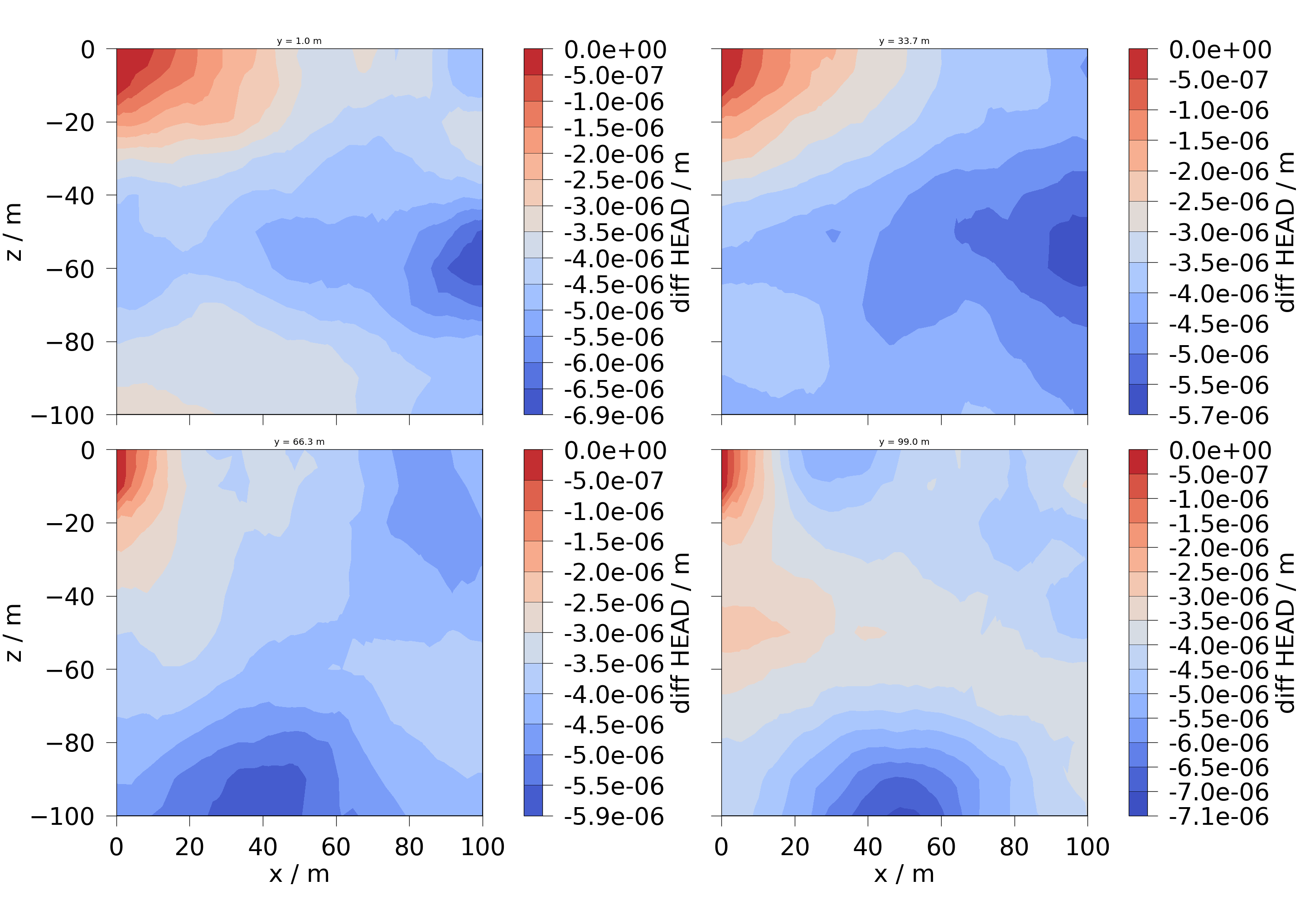
6.2 Slices are taken along the y-axis.

slices = np.reshape(
    list(feflow_model.mesh.slice_along_axis(n=4, axis="y")), (2, 2)
)
fig = ot.plot.contourf(slices, diff_head)
for ax, slice in zip(fig.axes, np.ravel(slices), strict=False):
    ax.set_title(f"y = {slice.center[1]:.1f} m", fontsize=32)