Plotting nuclear waste heat over time

Section author: Florian Zill (Helmholtz Centre for Environmental Research GmbH - UFZ)

First, some minimal example usage:

import matplotlib.pyplot as plt
import numpy as np

import ogstools.physics.nuclearwasteheat as nuclear

repo = nuclear.repo_2020_conservative
units = {"time_unit": "yrs", "power_unit": "kW"}  # default is s and W
print("Heat at start of deposition (1 nuclear waste bundle): ")
print(f"{0:6n} yrs: {repo.heat(t=0, **units):10.1f} kW")
print("Heat after deposition complete (all nuclear waste bundles): ")
print(
    f"{repo.time_deposit('yrs'):6n} yrs: "
    f"{repo.heat(t=repo.time_deposit('yrs'), **units):10.1f} kW"
)
print("Heat for a timeseries: ")
time = np.geomspace(1, 1e5, num=6)
heat = repo.heat(t=time, **units)
print(
    *[f"{t:6n} yrs: {q:10.1f} kW" for t, q in zip(time, heat, strict=False)],
    sep="\n",
)

Heat at start of deposition (1 nuclear waste bundle):
     0 yrs:        0.6 kW
Heat after deposition complete (all nuclear waste bundles):
    30 yrs:    16344.7 kW
Heat for a timeseries:
     1 yrs:      649.9 kW
    10 yrs:     6126.8 kW
   100 yrs:     8815.1 kW
  1000 yrs:     2011.2 kW
 10000 yrs:      480.1 kW
100000 yrs:       34.6 kW

Now for the plotting define the timeframe and heat models of interest. Also let’s make a convenience function to format our plots.

time = np.geomspace(1, 1e6, num=100)
models = [model for model in nuclear.waste_types if "2016" not in model.name]
ls = ["-", "--", "-.", ":", (0, (1, 10))]


def format_ax(ax: plt.Axes):
    ax.set_xlabel("time / yrs")
    ax.set_ylabel("heat / kW")
    ax.grid(True, which="major", linestyle="-")
    ax.grid(True, which="minor", linestyle="--", alpha=0.2)
    ax.legend()

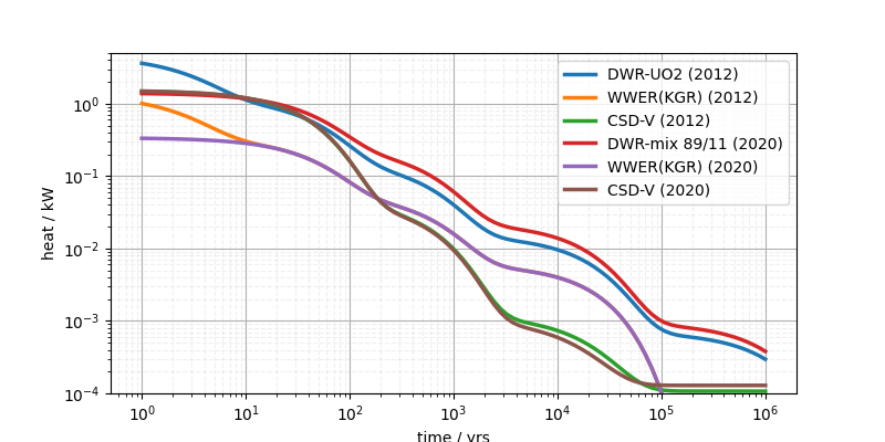
Let’s compare the heat timeseries of single containers of different nuclear waste types without interim storage or deposition taken into account (baseline=True).

fig, ax = plt.subplots(figsize=(8, 4))
for model in models:
    q = model.heat(time, baseline=True, **units)
    ax.loglog(time, q, label=model.name, lw=2.5)
format_ax(ax)
ax.set_ylim([1e-4, 5])
plt.show()

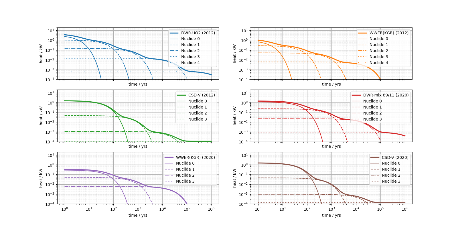
The bumps in the curves stem from the different leading nuclides in the proxy model sequentially decaying to nothing. The leading nuclides don’t necessarily represent actual physical nuclides, but they give a close match to the result of burn-off simulations. We can visualize the decay of the nuclides themselves as well:

fig, axs = plt.subplots(
    nrows=int(0.5 + len(models) / 2), ncols=2, figsize=(16, 8), sharex=True
)
axs: list[plt.Axes] = np.reshape(axs, (-1))

colors = plt.rcParams["axes.prop_cycle"].by_key()["color"]
for ax, model, color in zip(axs, models, colors, strict=False):
    q = model.heat(time, baseline=True, **units)
    ax.loglog(time, q, label=model.name, lw=2.5, c=color)
    for i in range(len(model.nuclide_powers)):
        q = model.heat(time, baseline=True, ncl_id=i, **units)
        ax.loglog(time, q, label=f"Nuclide {i}", lw=1.5, c=color, ls=ls[i])
    format_ax(ax)
    ax.set_ylim([1e-4, 20])
plt.show()

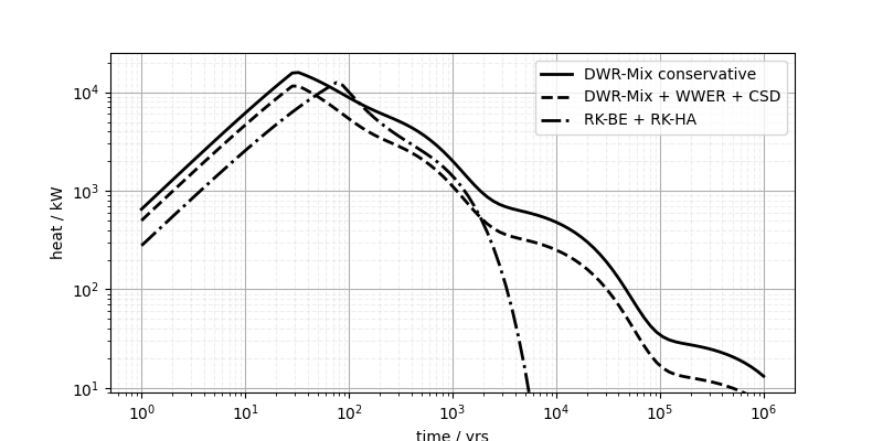
When taking the interim storage time and the time to fill the repository into account we get a linear increase of bundles adding to the total heat. Is is assumed, that each bundle has reached exactly the interim storage time at the moment it is deposited. Let’s compare the different available repository models.

fig, ax = plt.subplots(figsize=(8, 4))

repos = [
    nuclear.repo_2020_conservative,
    nuclear.repo_2020,
    nuclear.repo_be_ha_2016,
]
repo_heat = [repo.heat(time, **units) for repo in repos]
ax.loglog(time, repo_heat[0], "k", label="DWR-Mix conservative", lw=2, ls=ls[0])
ax.loglog(time, repo_heat[1], "k", label="DWR-Mix + WWER + CSD", lw=2, ls=ls[1])
ax.loglog(time, repo_heat[2], "k", label="RK-BE + RK-HA", lw=2, ls=ls[2])
format_ax(ax)
ax.set_ylim([9, 25000])
plt.show()

fig, ax = plt.subplots(figsize=(8, 2))

ax.loglog(time, repo_heat[0], label="DWR-Mix", lw=2, c="k")
for i in range(len(nuclear.repo_2020_conservative.waste[0].nuclide_powers)):
    q = nuclear.repo_2020_conservative.heat(time, ncl_id=i, **units)
    ax.loglog(time, q, label=f"Nuclide {i}", lw=1.5, c="k", ls=ls[i])
format_ax(ax)
ax.set_ylim([9, 25000])
plt.show()