Read mesh from file (vtu or xdmf) into pyvista mesh

import numpy as np

from ogstools import examples

To read your own data as a MeshSeries you can do:

from ogstools.meshlib import MeshSeries
mesh_series = MeshSeries("filepath/filename_pvd_or_xdmf")

MeshSeries takes as mandatory argument a str OR pathlib.Path that represents the location of the pvd or xdmf file. Here, we load example data and print the meta information:

ms = examples.load_meshseries_HT_2D_XDMF()
ms

<ogstools.meshlib.mesh_series.MeshSeries object at 0x7b2716a0f220>

Accessing time values

Time values (and spatial coordinates) can be unit transformed via scale(). Either pass a tuple to convert from the first to the second unit or pass a scaling factor.

print(f"First 3 time values are: {ms.timevalues[:3]} s.")
ms = ms.scale(time=("s", "h"))
print(f"Last time value is: {ms.timevalues[-1]} h.")
ms = ms.scale(time=3600.0)
print(f"Last time value is: {ms.timevalues[-1]} s.")

First 3 time values are: [   0.  900. 1800.] s.
Last time value is: 24.0 h.
Last time value is: 86400.0 s.

Accessing meshes

To get a single mesh at a specified timestep you can use the mesh() method of a MeshSeries object (in this example: ms). Another way to to do so is by indexing the MeshSeries object with brackets (ms[timestep]). Besides custom ogstools functions you can use all available pyvista functions. Here we use pyvista’s plot function.

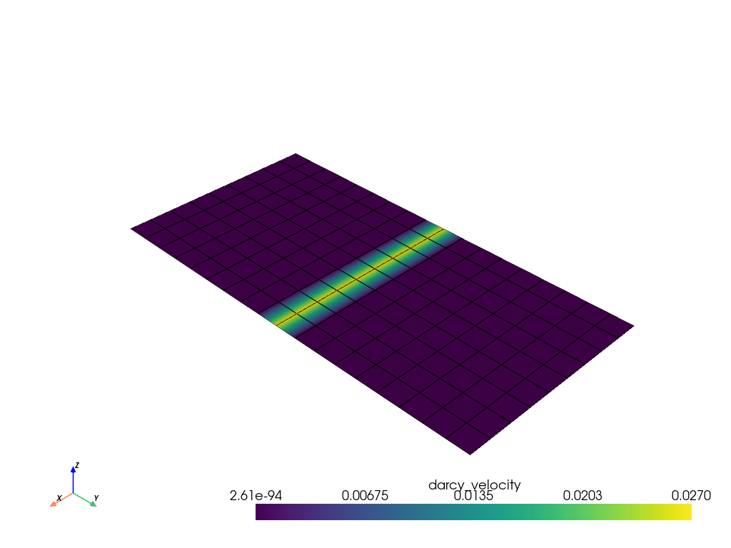
mesh_ts10 = ms.mesh(10)  # or ms[10]
mesh_ts10.plot(show_edges=True)

Static Scene

Interactive Scene

Indexing

MeshSeries.values(“<variable_name>”)` returns a numpy ndarray. It allows multidimensional indexing on ndarrays.

Typically, the first dimension is the time step, second dimension is the number of points/cells, and the last dimension is the number of components of the variable.

By default, values would read the entire dataset. If only a subset of the MeshSeries should be read you can select the relevant timesteps by indexing / slicing the MeshSeries directly. This selection will also be adhered to if you read individual meshes.

ms = examples.load_meshseries_HT_2D_XDMF()
# Temperature is a scalar, Darcy velocity is a vector with 2 components.
# Both are defined at points.

print("Entire dataset:", np.shape(ms.values("temperature")))
print("Every second timestep:", np.shape(ms[::2].values("temperature")))
print("Last two steps:", np.shape(ms[-2:].values("darcy_velocity")))

Entire dataset: (97, 190)
Every second timestep: (49, 190)
Last two steps: (2, 190, 2)

To select points or cells you can use the extract method to specify the corresponding ids.

temp_at_points = ms.extract([2, 3, 4]).values("temperature")
print("Data on extracted points:", np.shape(temp_at_points))
print("Temperatures at last timestep:", temp_at_points[-1])

Data on extracted points: (97, 3)
Temperatures at last timestep: [352.9994477  303.         353.00000001]

You can also use pyvista dataset filters to transform the domain for the entire MeshSeries.

ms_right_half = ms.transform(
    lambda mesh: mesh.clip("x", mesh.center, crinkle=True)
)
temp_right_half = ms_right_half.values("temperature")
print("Data on clipped domain:", np.shape(temp_right_half))

Data on clipped domain: (97, 114)

Let’s plot the last timestep of the transformed MeshSeries.

fig = ms_right_half[-1].plot_contourf("temperature")