How to plot data at observation points

Section author: Florian Zill (Helmholtz Centre for Environmental Research GmbH - UFZ)

In this example we plot the data values on observation points over all timesteps. Since requested observation points don’t necessarily coincide with actual nodes of the mesh different interpolation options are available. See ogstools.meshlib.mesh_series.MeshSeries.probe for more details. Here we use a component transport example from the ogs benchmark gallery (https://www.opengeosys.org/docs/benchmarks/hydro-component/elder/).

import matplotlib.pyplot as plt
import numpy as np

import ogstools as ot
from ogstools import examples

mesh_series = examples.load_meshseries_CT_2D_XDMF().scale(time=("s", "a"))
si = ot.variables.saturation

To read your own data as a mesh series you can do:

from ogstools.meshlib import MeshSeries
mesh_series = MeshSeries("filepath/filename_pvd_or_xdmf")

You can also use a variable from the available presets instead of needing to create your own: Variable presets and data transformation

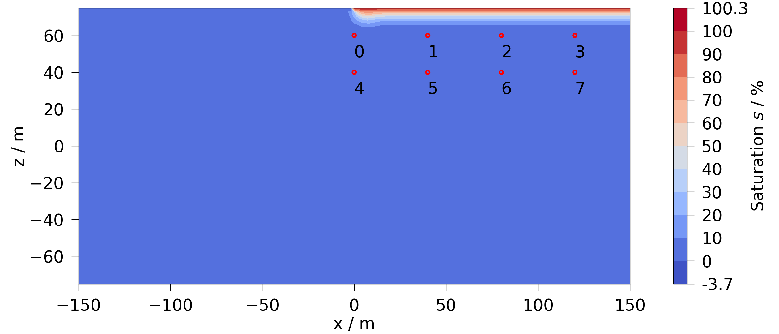
Let’s define 4 observation points and plot them on the mesh.

rows = np.array([np.linspace([0, 0, z], [120, 0, z], 4) for z in [60, 40]])
fig = mesh_series.mesh(0).plot_contourf(si)
fig.axes[0].scatter(rows[..., 0], rows[..., 2], s=50, fc="none", ec="r", lw=3)
for i, pt in enumerate(rows.reshape(-1, 3)):
    fig.axes[0].annotate(str(i), (pt[0], pt[2] - 5), va="top", fontsize=32)

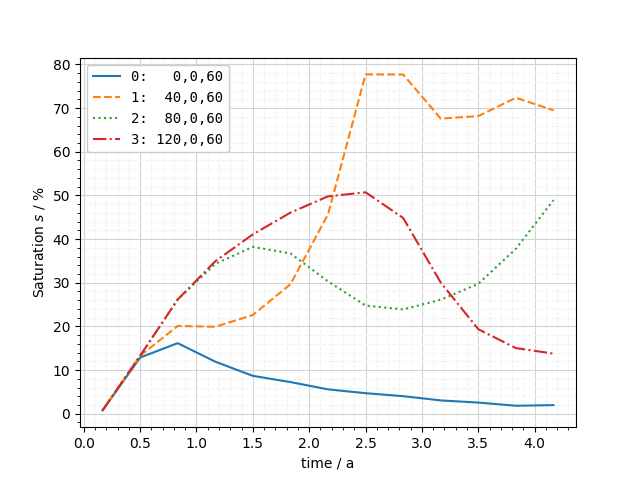
And now probe the points and plot the values over time.

labels = [
    [f"{i}: x={pt[0]: >5} z={pt[2]}" for i, pt in enumerate(pts)]
    for pts in rows
]
ms_pts = [ot.MeshSeries.extract_probe(mesh_series, pts) for pts in rows]
fig = ot.plot.line(ms_pts[0], "time", si, labels=labels[0], monospace=True)

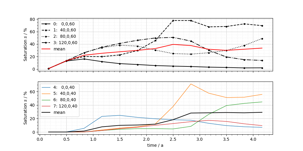
You can also pass create your own matplotlib figure and pass the axes object. Additionally, you can pass any keyword arguments which are known by matplotlibs plot function to further customize the curves. To show, how to customize a plot afterwards, we add the mean saturation of the 4 observation points per row to each subplot.

fig, axs = plt.subplots(nrows=2, figsize=[16, 10], sharey=True)
ot.plot.line(ms_pts[0], "time", si, ax=axs[0], color="k", fontsize=20)
ot.plot.line(ms_pts[1], "time", si, ax=axs[1], marker="o", fontsize=20)
# add the mean of the observation point timeseries
for index in range(2):
    values = si.transform(ms_pts[index])
    mean_values = np.mean((values), axis=-1)
    ts = ms_pts[index].timevalues
    fig.axes[index].plot(ts, mean_values, "rk"[index], lw=4)
    fig.axes[index].legend(labels[index] + ["mean"], fontsize=20)