How to compare results with reference data or an analytical solution

Section author: Florian Zill (Helmholtz Centre for Environmental Research GmbH - UFZ)

This example provides recipes for frequently needed plots in the OpenGeoSys benchmark section. It is a repeating pattern, to compare numerical results with analytical or reference data and evaluate the errors. The goal here is to have a standardized recipe for cleaner code and less repetition.

import matplotlib.pyplot as plt
import numpy as np

import ogstools as ot
from ogstools import examples

temp = ot.variables.temperature

Compute the analytical solution

Note, that the relative errors are calculated with the reference values in data units, i.e. in Kelvin.

results = examples.load_meshseries_diffusion_3D()
x = results[0].points[:, 0]
analytical_func = examples.anasol.heat_conduction_temperature

ref_values = np.asarray([analytical_func(x, tv) for tv in results.timevalues])
abs_error = ref_values - results["temperature"]
rel_error = abs_error / ref_values
np.testing.assert_array_less(np.abs(abs_error), 6)
np.testing.assert_array_less(np.abs(rel_error), 0.02)
results = results.scale(time=("s", "h"))

Write the data into the results, to leverage plotting features.

results.point_data[temp.anasol.data_name] = ref_values
results.point_data[temp.abs_error.data_name] = abs_error
results.point_data[temp.rel_error.data_name] = rel_error

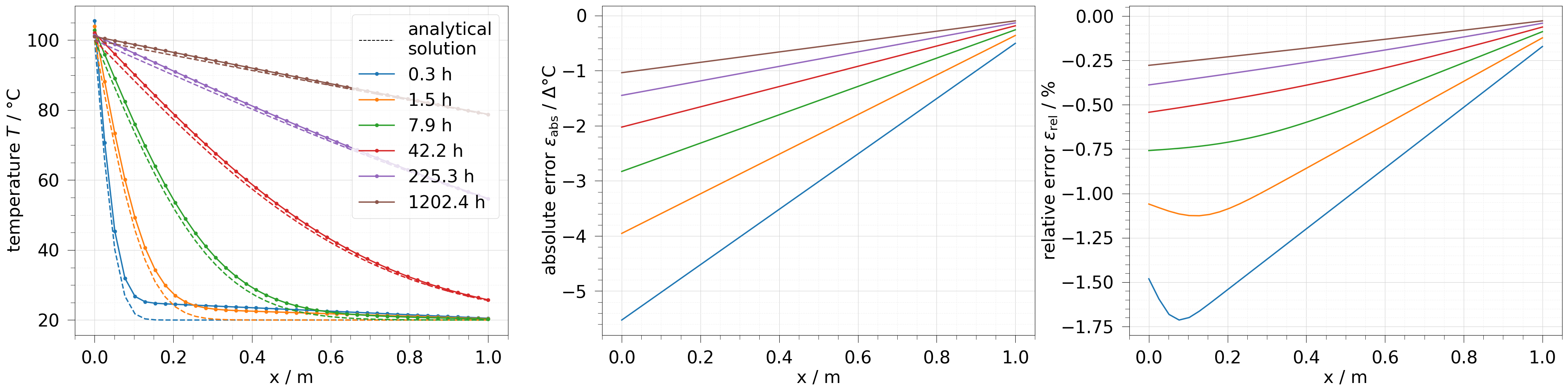
Comparing data over a line for multiple timesteps

If the resulting data is not already one-dimensional we need to extract the points which make up the line of interest. We can do so, by using extract and the point indices or by using extract_probe and a set of points. We need to further select the timesteps we want to plot. This is done by indexing the MeshSeries object.

fig, axs = plt.subplots(1, 3, figsize=[40, 10])
# extract every second timestep and only the points on the x-axis
x_edge = results[::2].extract(
    (results[0].points[:, 1] == 0) & (results[0].points[:, 2] == 0)
)
labels = [f"{tv:.1f} h" for tv in x_edge.timevalues]
axs[0].plot([], [], "--k", label="analytical\nsolution")
ot.plot.line(x_edge, temp, ax=axs[0], marker="o", labels=labels)
ot.plot.line(x_edge, temp.anasol, ax=axs[0], ls="--")
ot.plot.line(x_edge, temp.abs_error, ax=axs[1])
ot.plot.line(x_edge, temp.rel_error, ax=axs[2])
fig.tight_layout()

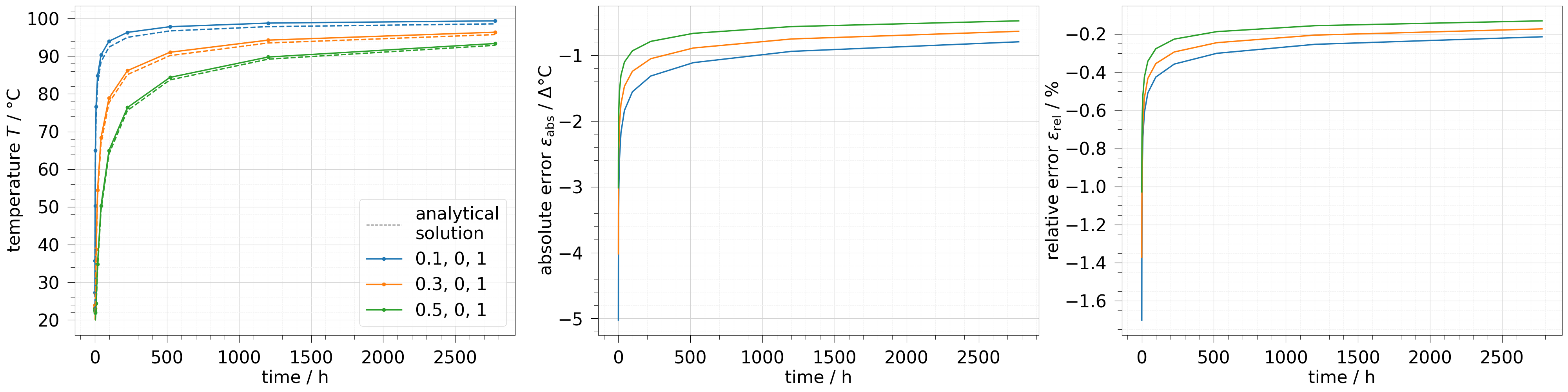
Comparing data of multiple points over time

Here, we use the same strategy as before, but in the plot.line function, we specify, that we want to plot over the time dimension.

fig, axs = plt.subplots(1, 3, figsize=(40, 10))
pts = np.asarray([[0.1, 0, 1], [0.3, 0, 1], [0.5, 0, 1]])
probe = ot.MeshSeries.extract_probe(results, pts)
labels = ot.plot.utils.justified_labels(pts)
axs[0].plot([], [], "--k", label="analytical\nsolution")
ot.plot.line(probe, "time", temp, ax=axs[0], marker="o", labels=labels)
ot.plot.line(probe, "time", temp.anasol, ax=axs[0], ls="--")
ot.plot.line(probe, "time", temp.abs_error, ax=axs[1])
ot.plot.line(probe, "time", temp.rel_error, ax=axs[2])
fig.tight_layout()

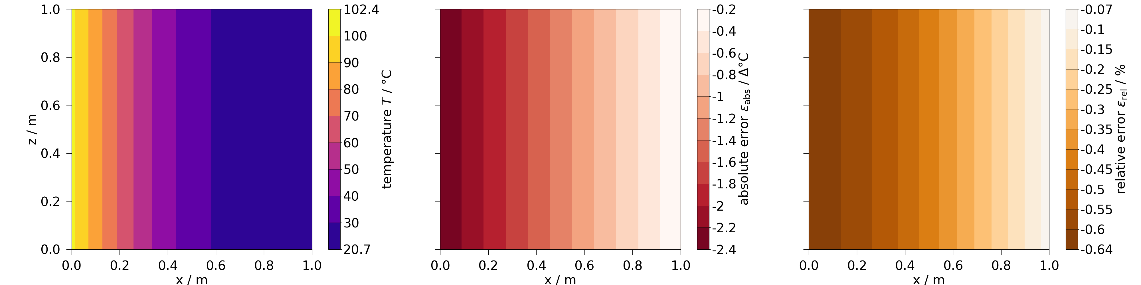
Comparing data of a 2D slice in a contourplot

Again, we prepare the results, by extract the 2D data, we want to inspect. This can be done by slicing the original 3D results and selecting the timestep of interest.

fig, axs = plt.subplots(1, 3, figsize=[40, 10], sharey=True)
results_y_slice = results.transform(lambda mesh: mesh.slice("y"))
y_slice = results_y_slice[results.closest_timestep(20)]
y_slice.plot_contourf(temp, fig=fig, ax=axs[0])
y_slice.plot_contourf(temp.abs_error, fig=fig, ax=axs[1])
y_slice.plot_contourf(temp.rel_error, fig=fig, ax=axs[2])
fig.tight_layout()

Comparing the transient data of a line

Here, we extract a line and plot a timeslice, to evaluate the data spatially and temporally.

fig, axs = plt.subplots(1, 3, figsize=[40, 10], sharey=True)

x_edge = results.extract(
    (results[0].points[:, 1] == 0) & (results[0].points[:, 2] == 0)
)
x_edge.plot_time_slice("x", "time", temp, fig=fig, ax=axs[0])
x_edge.plot_time_slice("x", "time", temp.abs_error, fig=fig, ax=axs[1])
x_edge.plot_time_slice("x", "time", temp.rel_error, fig=fig, ax=axs[2])
fig.tight_layout()

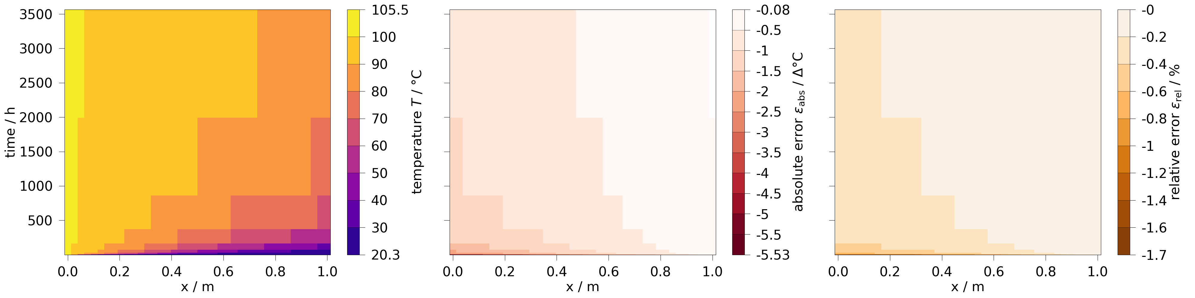
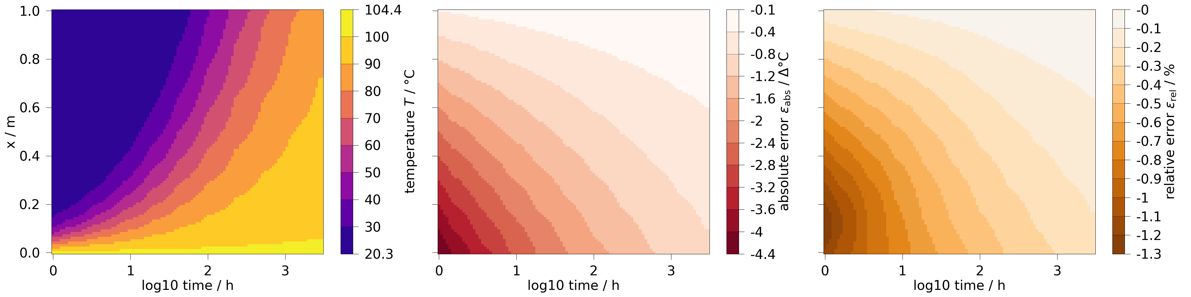
We can also increase the resolution, by using a large number of probing points and by resampling with more timesteps. Using a logarithmic scaling for the time is beneficial here, as most of the changes in the results happen in the very beginning.

fig, axs = plt.subplots(1, 3, figsize=[40, 10], sharey=True)
line_pts = np.linspace([0, 0, 0], [1, 0, 0], num=100)
ms_line = ot.MeshSeries.extract_probe(results, line_pts)
ms_line = ot.MeshSeries.resample(ms_line, np.geomspace(1, 3000, num=100))
for i, var in enumerate([temp, temp.abs_error, temp.rel_error]):
    ms_line.plot_time_slice(
        "time", "x", var, fig=fig, ax=axs[i], time_logscale=True
    )
fig.tight_layout()