

Note
Go to the end to download the full example code or to run this example in your browser via Binder.
Visualizing 2D model data#
To demonstrate the creation of filled contour plots we load a 2D THM meshseries
example. In the plot.setup we can provide a dictionary to map names
to material ids. Other plot configurations are also available, see:
ogstools.plot.plot_setup.PlotSetup. Some of these options are also
available as keyword arguments in the function call. Please see
ogstools.plot.contourplots.contourf for more information.
import ogstools as ot
from ogstools import examples

ot.plot.setup.material_names = {i + 1: f"Layer {i+1}" for i in range(26)}
ms = examples.load_meshseries_THM_2D_PVD().scale(spatial="km")
mesh = ms.mesh(1)
To read your own data as a mesh series you can do:
mesh_series = ot.MeshSeries("filepath/filename_pvd_or_xdmf", "km")
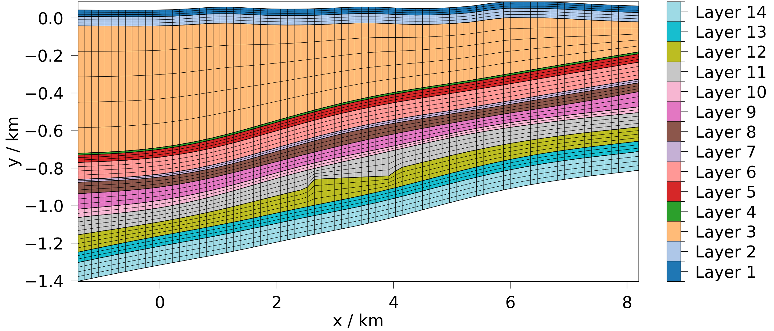
Plotting Cell Data#
First, let’s plot the material ids, which is part of the mesh’s cell_data. Per default in the setup, this will automatically show the element edges.
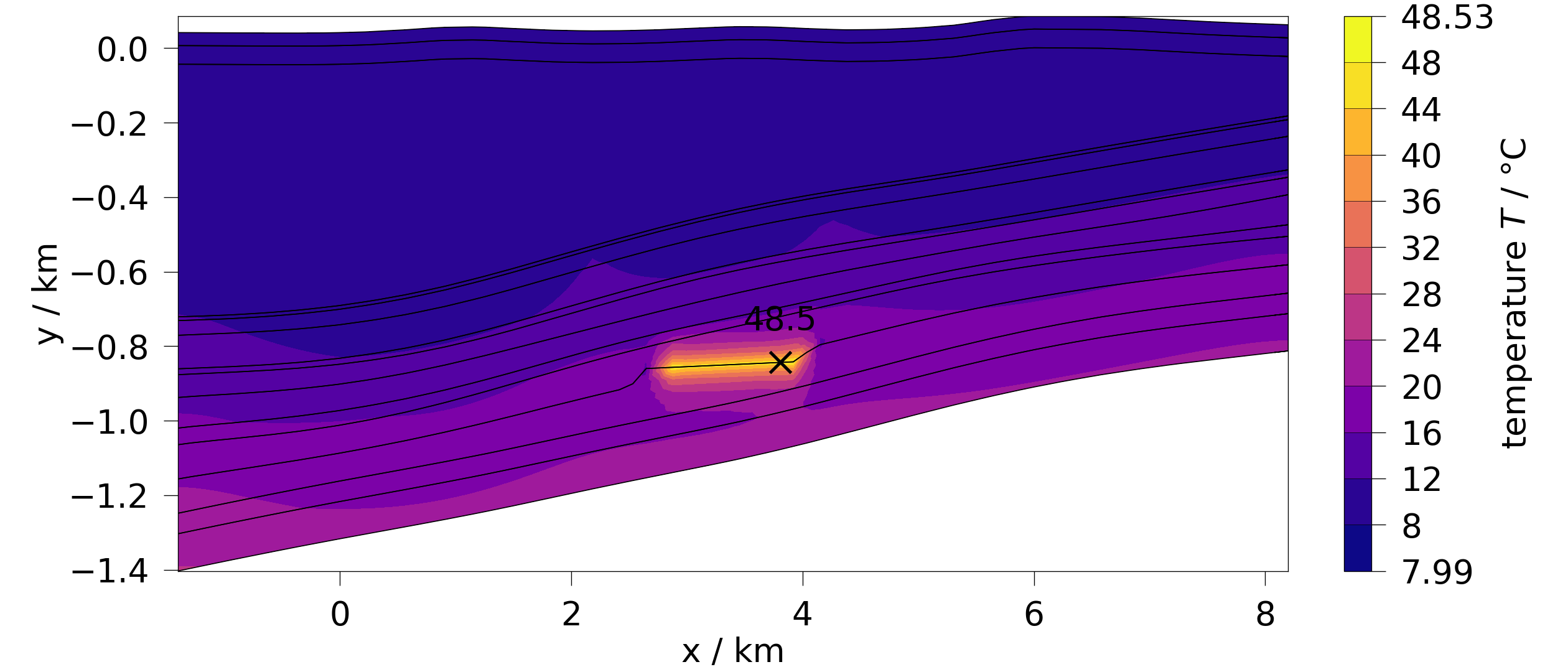
Plotting Point Data#
Now, let’s plot the temperature field (point_data) at the first timestep.
The default temperature variable from the variables reads the temperature
data as Kelvin and converts them to degrees Celsius. This also shows how to
only plot a specific part of the model by creating a clip with
pyvista.clip_box beforehand.
part = mesh.clip_box(bounds=[2, 5, -1.1, -0.7, 6, 7], invert=False)
fig = ot.plot.contourf(part, ot.variables.temperature, show_max=True)
We can also plot components of vector variables:
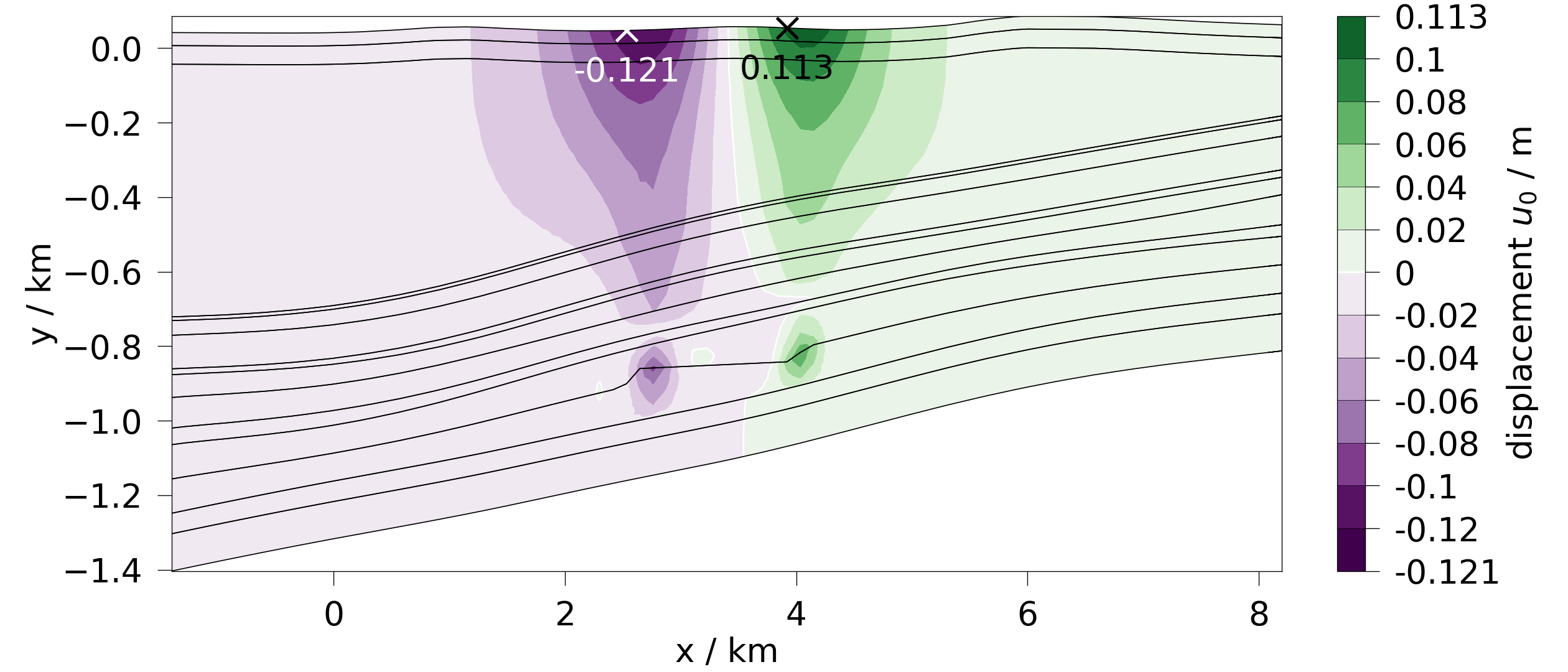
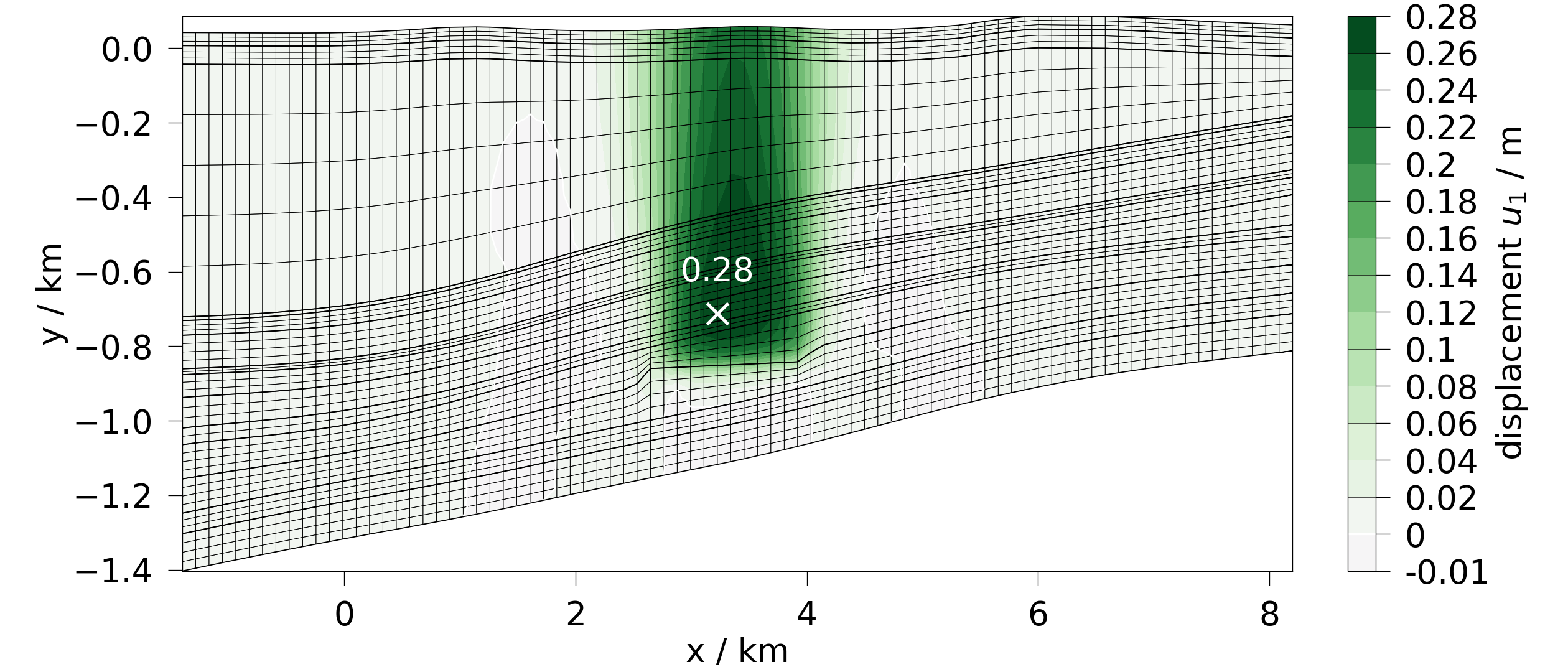
To have a continuous colormap instead of discrete colors per level pass a the equally named argument. In this case this helps to increase the level of detail of the negative displacements due to the bilinear colormap. You are also able to access the vector component via a string of the data with the appended suffix.
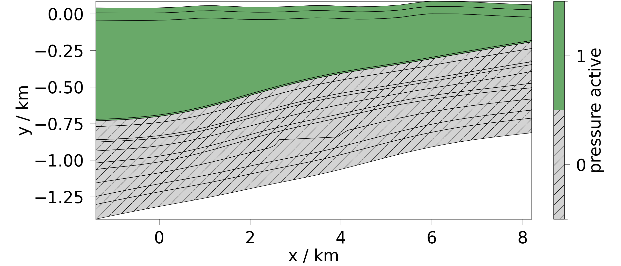
Plotting with deactivated subdomains#
This example has hydraulically deactivated subdomains, which will mask the related variables.
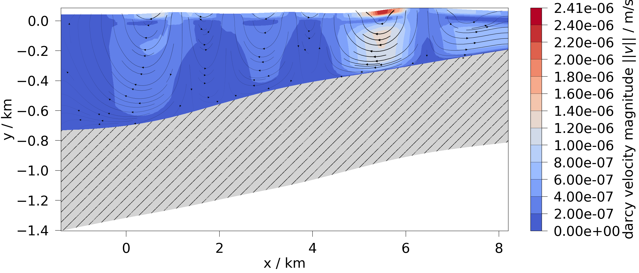
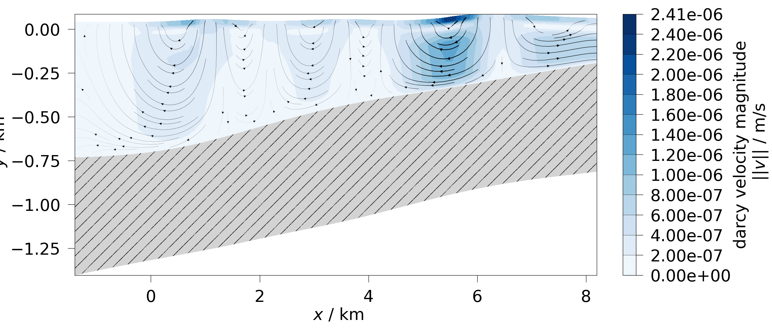
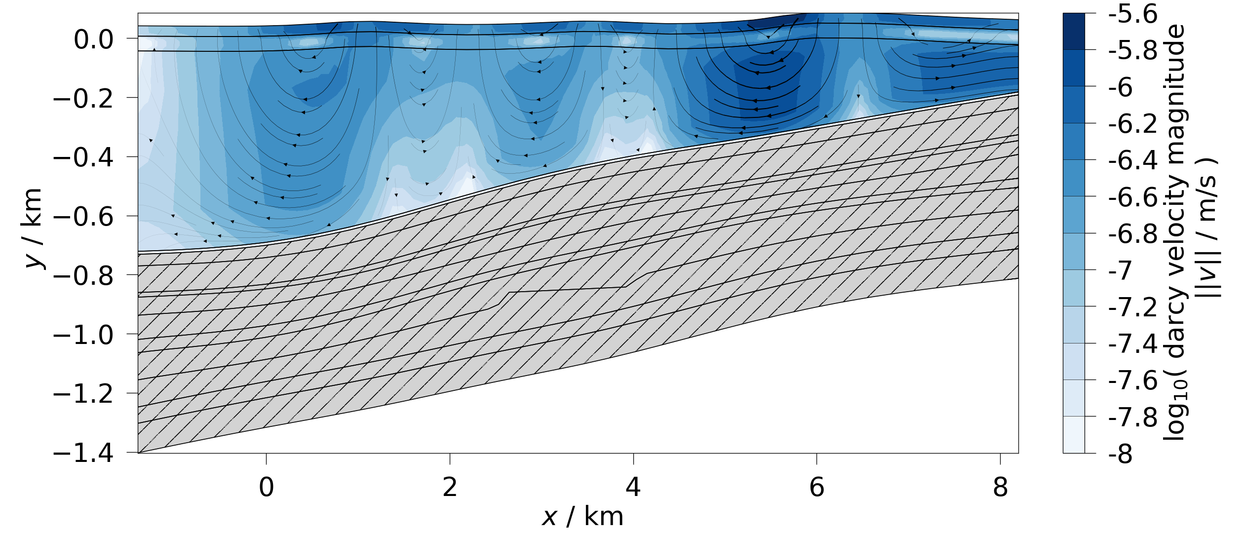
Plotting vector data#
Let’s plot the fluid velocity field. As this is vectorial data, this will automatically add streamlines to indicate the vector directions.
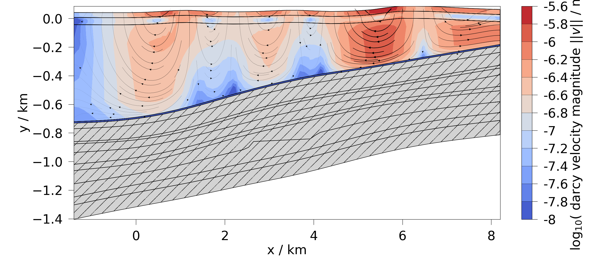
Let’s plot it again, this time log-scaled.
Total running time of the script: (0 minutes 7.822 seconds)