Aggregation of Meshseries Data

Section author: Florian Zill (Helmholtz Centre for Environmental Research GmbH - UFZ)

In this example we show how to aggregate data in a model over all timesteps as well as plot differences between to timesteps. For this purpose we use a component transport example from the ogs benchmark gallery (https://www.opengeosys.org/docs/benchmarks/hydro-component/elder/).

To see this benchmark results over all timesteps have a look at How to create Animations.

import numpy as np

import ogstools as ot
from ogstools import examples

mesh_series = examples.load_meshseries_CT_2D_XDMF().scale(time=("s", "a"))
saturation = ot.variables.saturation

To read your own data as a mesh series you can do:

from ogstools.meshlib import MeshSeries
mesh_series = MeshSeries("filepath/filename_pvd_or_xdmf")

You can also use a variable from the available presets instead of needing to create your own: Variable presets and data transformation

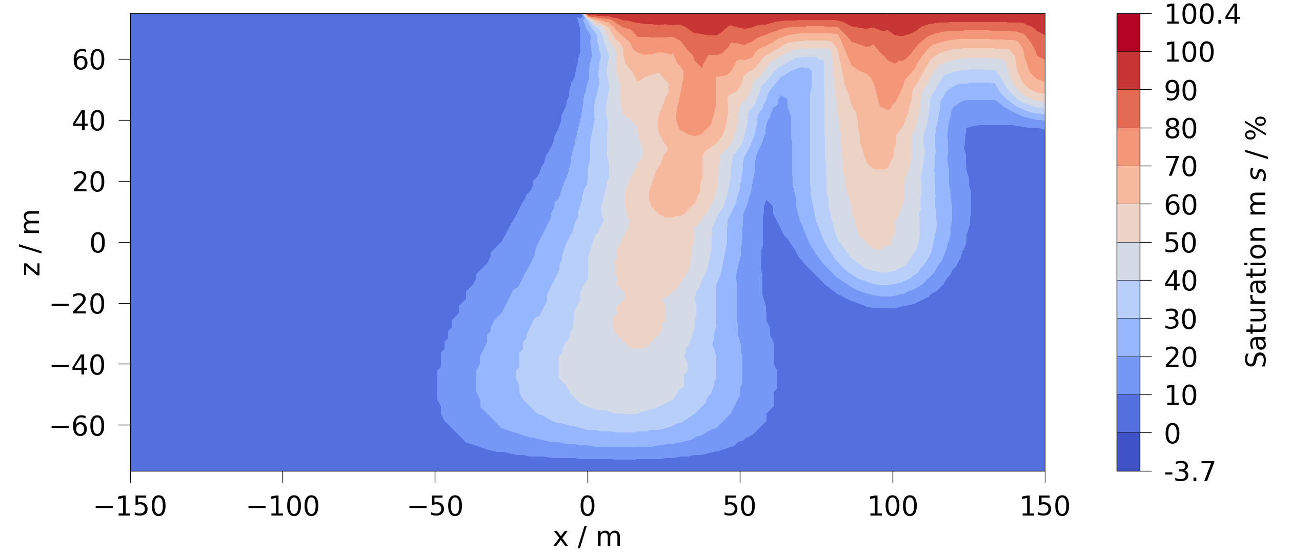
You aggregate the data in MeshSeries over all timesteps given some aggregation function, e.g. np.min, np.max, np.var (see: aggregate_over_time()). The following code gets the maximum saturation for each point in the mesh over all timesteps and plots it. Note: the data in the returned mesh has a suffix equal to the aggregation functions name. The plot function will find the correct data anyway if given the original variable

mesh = mesh_series.aggregate_over_time(saturation, np.max)
fig = mesh.plot_contourf(saturation)

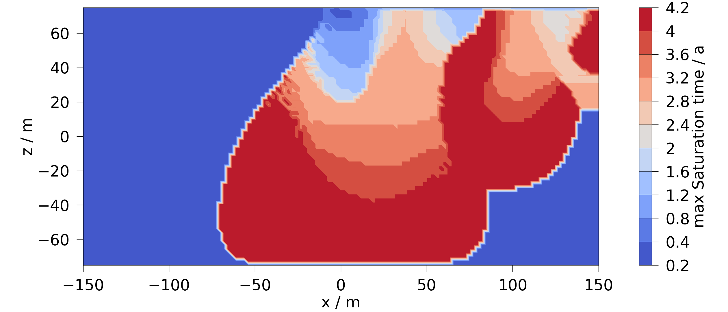
It is also possible to plot the time when the minimum or maximum occurs. However, here we have to use a new variable for the plot to handle the units correctly:

mesh = mesh_series.time_of_max(saturation)
fig = mesh.plot_contourf(ot.variables.Scalar("max_Saturation_time", "a", "a"))

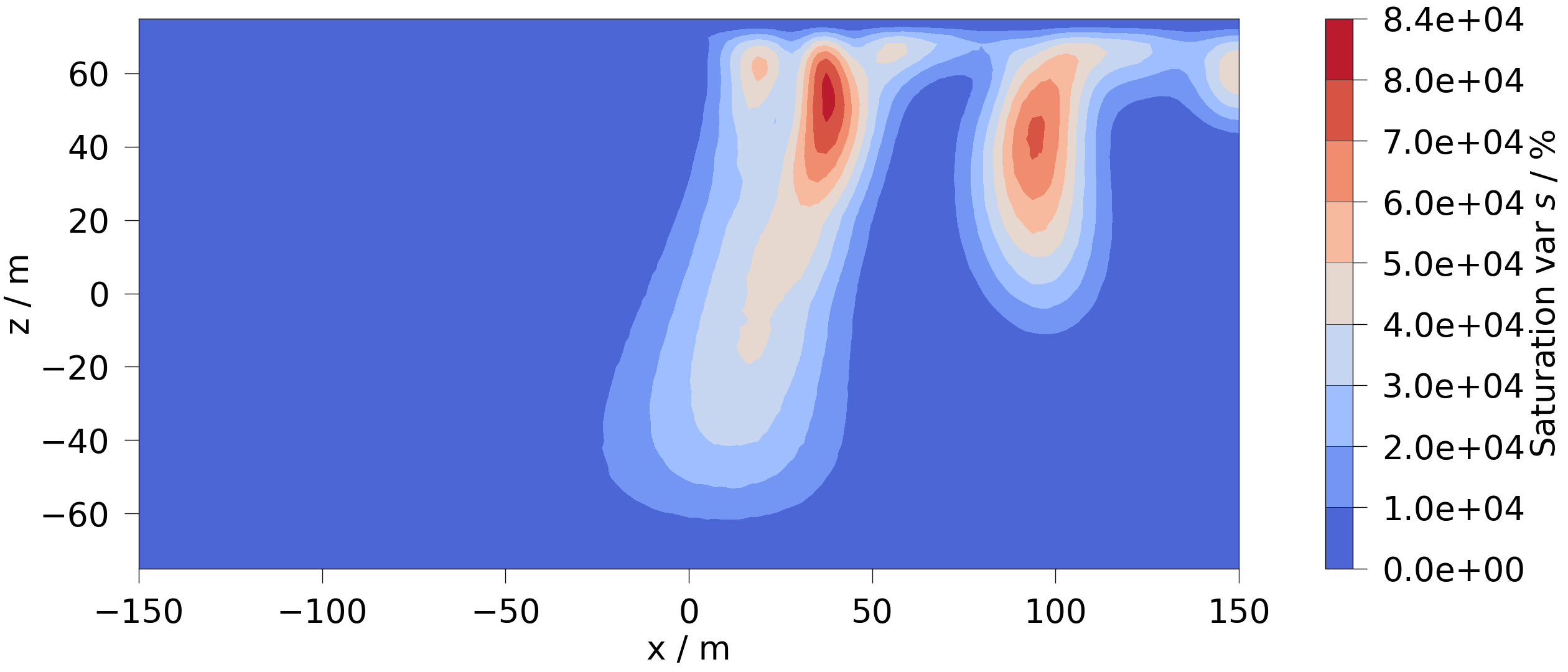
Likewise we can calculate and visualize the variance of the saturation:

mesh = mesh_series.aggregate_over_time(saturation, np.var)
fig = mesh.plot_contourf(saturation)

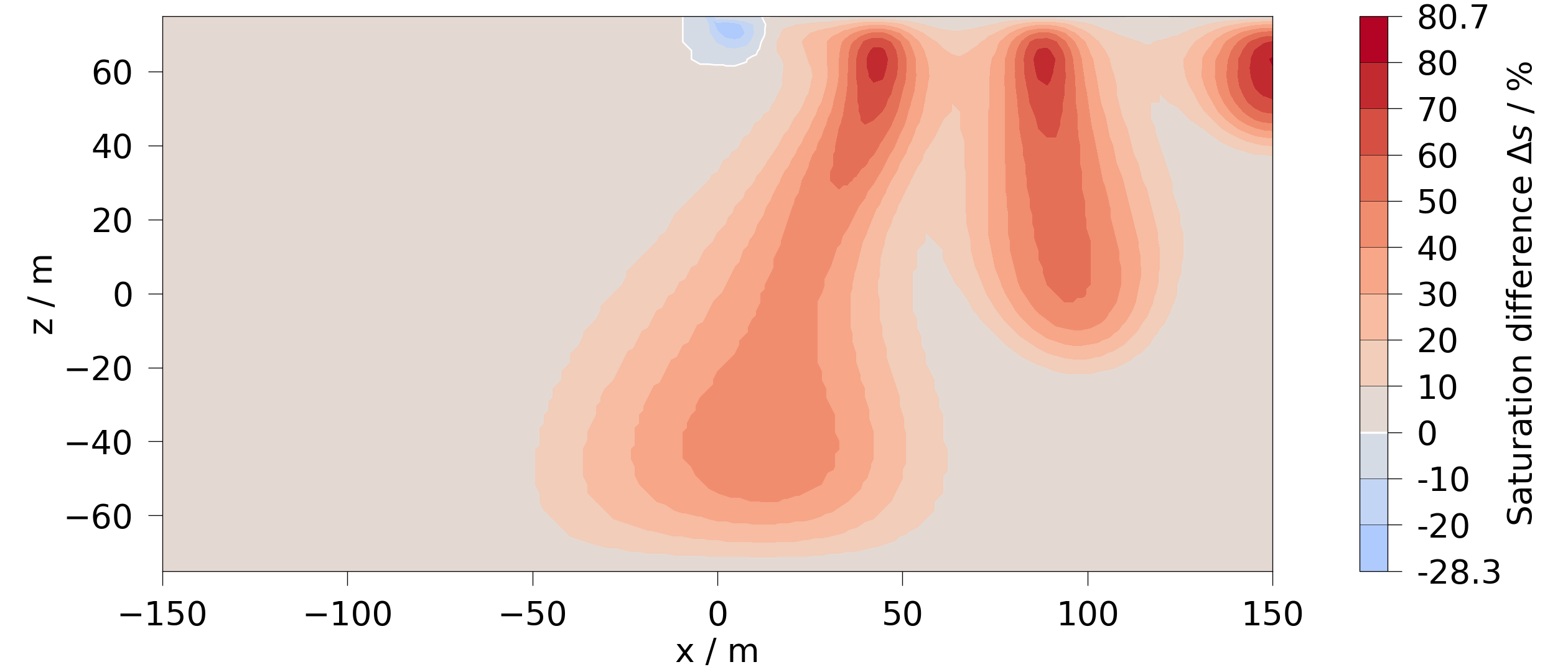
Difference between the last and the first timestep:

mesh = mesh_series.mesh(-1).difference(mesh_series.mesh(0), saturation)
fig = mesh.plot_contourf(saturation)

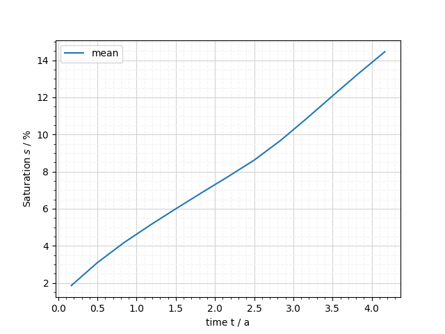
It’s also possible to aggregate the data per timestep to return a timeseries of e.g. the max or mean value of a variable in the entire domain.

fig = mesh_series.plot_domain_aggregate(saturation, np.mean)