Interactive Mesh manipulation (OGSTools - Integrated)

We demonstrate how to access and modify in situ meshes during an OpenGeoSys simulation.

Key features in this tutorial:

• Inspect mesh data via standard PyVista functions

• Dynamically modify point/cell properties (e.g., boundary conditions)

• React to simulation progress or state in an adaptive simulation loop

This tutorial builds on the Run a simulation - Step by step. For a lower-level control, see Interactive Mesh manipulation (Native interface).

Imports and definitions

%%

from pathlib import Path
from tempfile import mkdtemp
from time import sleep  # For simulation pause / interrupt

import numpy as np

import ogstools as ot
from ogstools.examples import load_model_liquid_flow_simple
from ogstools.simulation import SimulationController

Select a Project

We will start with a simple liquid flow project.

working_dir = Path(mkdtemp())
prj, meshes = load_model_liquid_flow_simple()
prj.write_input(working_dir / "LiquidFlowSimple.prj")
_ = meshes.save(working_dir)

Read and write in situ meshes

We will work with these functions:

• ot.Mesh.from_simulator

  gives you direct access to the values of th in situ-Mesh during a running OGS simulation

• SimulationController, that works exactly like OGSSimulation introduced in Run a simulation - Step by step.

This example demonstrates an adaptive simulation loop:

1. The simulation is monitored for steady-state convergence

2. Boundary conditions are dynamically adjusted during runtime

sim2_result_dir = working_dir / "sim2"
sim2_result_dir.mkdir(exist_ok=True)
arguments = [
    "",
    str(working_dir / "LiquidFlowSimple.prj"),
    "-o",
    str(sim2_result_dir),
]
sim2 = SimulationController(
    arguments
)  # we will restart the same simulation as above into new folder
domain_mesh = ot.Mesh.from_simulator(sim2, "domain", ["pressure"])

# Let us store the mesh of a time step to compare it later
previous_domain_mesh_pressure = domain_mesh.point_data["pressure"]
domain_mesh_pressure = previous_domain_mesh_pressure

# Later, we will dynamically modify the left boundary mesh
left_mesh = ot.Mesh.from_simulator(sim2, "left", ["pressure"])

steady_state_threshold = 0.1 * len(previous_domain_mesh_pressure)  # constant
delta = steady_state_threshold + 1e-10  # to be computed for each time step

Main simulation loop

The simulation is advanced step-by-step until either:

• The simulation reaches the defined end time, or

• The user interrupts execution (Ctrl+C or Stop the Jupyter cell)

while (
    sim2.current_time() < sim2.end_time()
    and not sim2.is_interrupted()
    # any other stopping condition based on the mesh, log, ...
    # e.g. # `delta > steady_state_threshold``
):

    previous_domain_mesh_pressure = domain_mesh.point_data["pressure"].copy()

    sim2.execute_time_step()
    sleep(0.01)  # Must have, if you want to pause the simulation

    # --------------- until here minimal loop -------------------------------
    # Example for an In-loop condition
    # 1. Check, if a steady state is reached
    # 2. Change a boundary condition

    delta = np.max(
        np.absolute(
            domain_mesh.point_data["pressure"] - previous_domain_mesh_pressure
        )
    )
    if delta < steady_state_threshold:
        print(
            "The steady state condition is reached. Now a new boundary condition is applied."
        )
        # [:] Is important! Otherwise you would assign a new numpy array to pressure (which would write into the in situ mesh)
        left_mesh.point_data["pressure"][:] = np.full(left_mesh.n_points, 3.1e7)
    # else: we keep the boundary conditions constant

# This simulation reaches the steady state condition twice
# 1st with left boundary pressure at 2.9e7 Pa, 2nd: 3.1e7 Pa

The steady state condition is reached. Now a new boundary condition is applied.

Intermediate plot

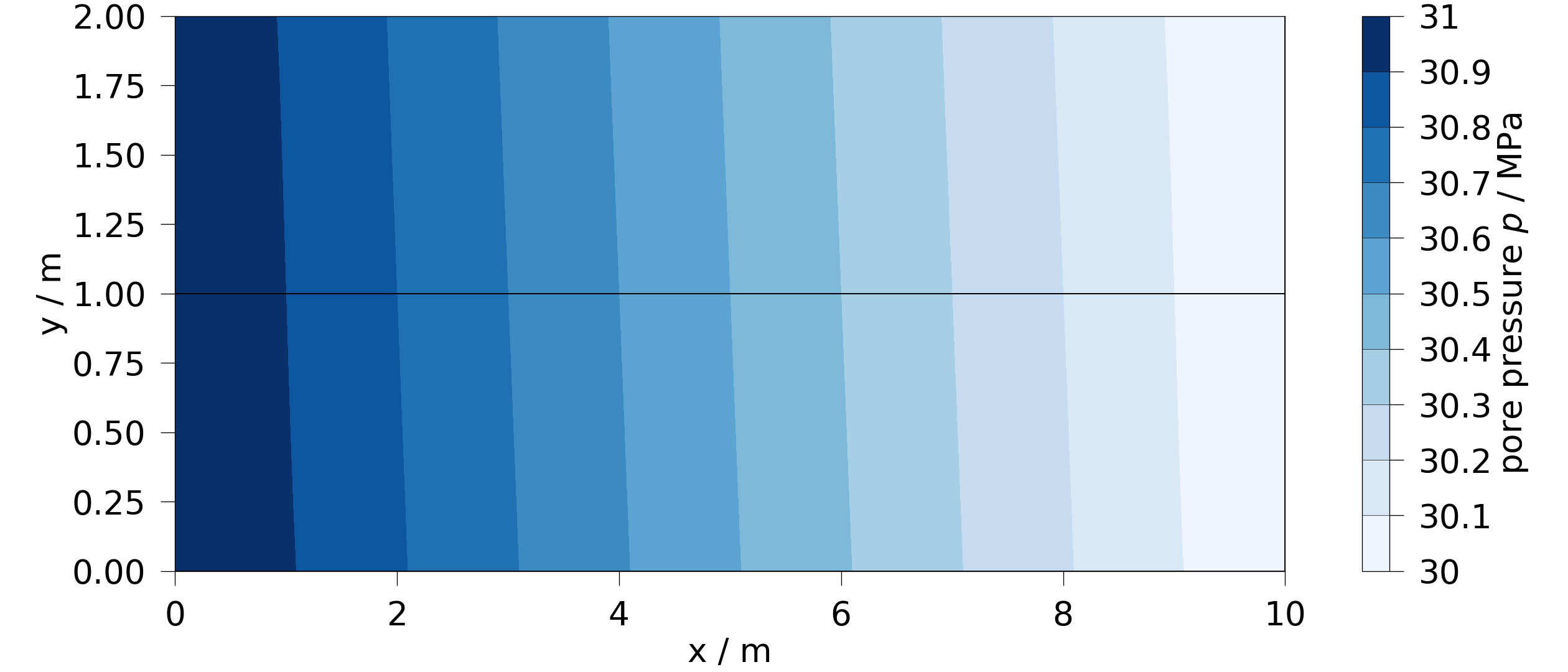
If the simulation is paused or interrupted, you can inspect the current state of the mesh. You are free to adapt the mesh and continue the simulation as shown in while loop above. Let us just plot the pressure field.

fig = ot.plot.contourf(domain_mesh, "pressure")

Continue the (“paused”) simulation

sim2.execute_time_step()
# Or run over multiple steps (see while loop above)
sim2.execute_simulation()
# Necessary to close, otherwise you can not reinitialize simulation with same prj-file (arguments)
sim2.close()

Visualization

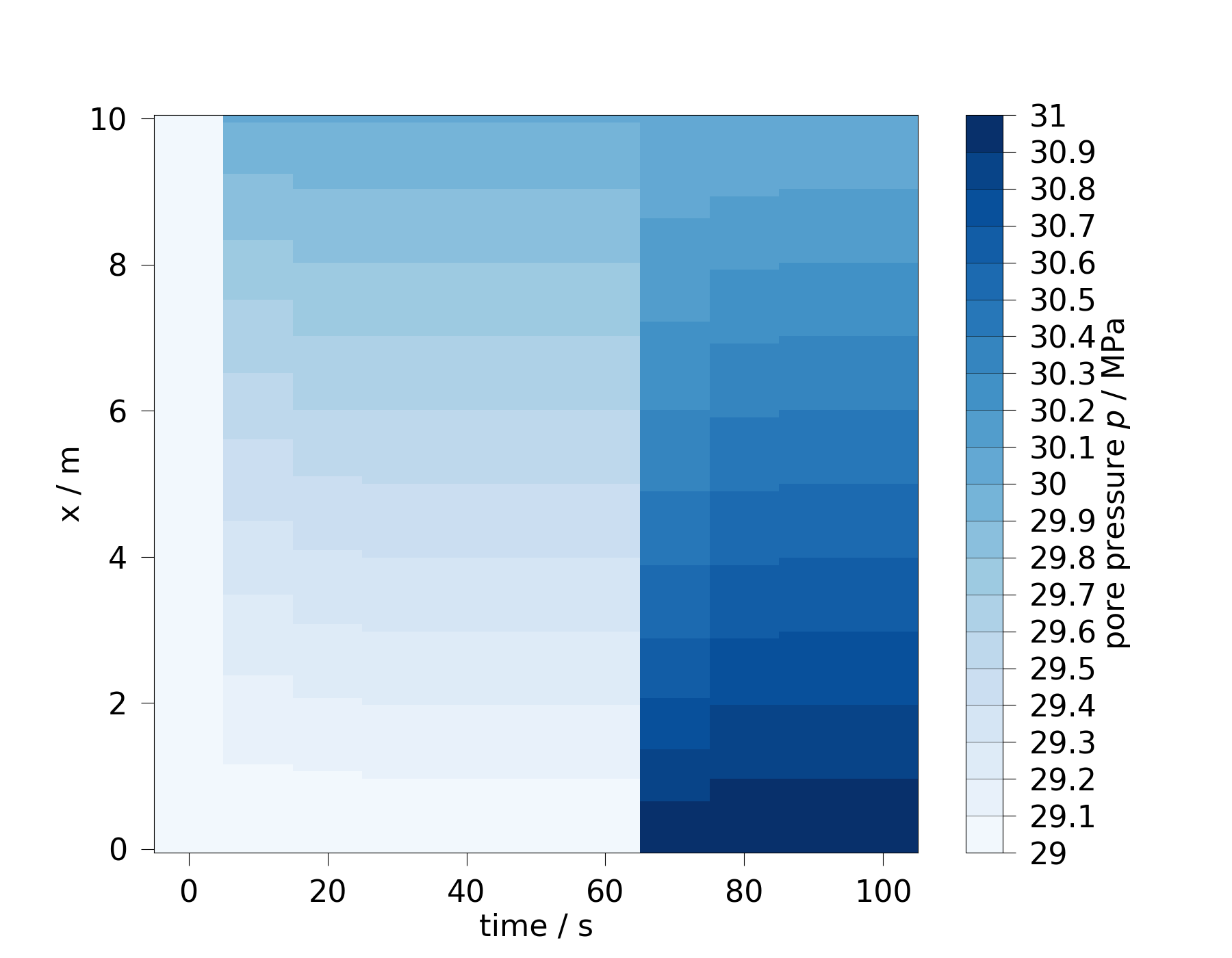
# We visualize how the dynamically updated boundary conditions affected the pressure field.
# Changes in boundary conditions can be clearly observed.
ms = ot.MeshSeries(sim2_result_dir / "LiquidFlow_Simple.pvd")
# !paraview {ms.filepath} # for interactive exploration
# Time slice over x
points = np.linspace([0, 1, 0], [10, 1, 0], 100)
ms_probe = ot.MeshSeries.extract_probe(ms, points, "pressure")
fig = ms_probe.plot_time_slice("time", "x", variable="pressure", num_levels=20)

  0%|          | 0/11 [00:00<?, ?it/s]
100%|██████████| 11/11 [00:00<00:00, 553.20it/s]

Note: Alternatively, for boundary conditions only (no interaction), have a look at our guide about Defining boundary conditions with Python.