

Note
Go to the end to download the full example code or to run this example in your browser via Binder.
Spatial & temporal refinement - nuclear decay#
This example shows one possible implementation of how to do a convergence study
with spatial and temporal refinement. For this, a simple model using a time
dependent heat source on one side and constant temperature on the opposite side
was set up. The heat source is generated with the
ogstools.physics.nuclearwasteheat model.
Here is some theoretical background for the topic of grid convergence:
At least three meshes from simulations of increasing refinement are required for the convergence study. The third finest mesh is chosen per default as the topology to evaluate the results on.
The results to analyze are generated on the fly with the following code. If you are only interested in the convergence study, please skip to Temperature convergence at maximum heat production (t=30 yrs).
First, the required packages are imported and a temporary output directory is created:
import matplotlib.pyplot as plt
import numpy as np
from IPython.display import HTML
from scipy.constants import Julian_year as sec_per_yr

import ogstools as ot
from ogstools import examples, physics, studies, workflow

temp_path = ot.definitions.temp_dir("nuclear_decay", "examples")
Let’s run the different simulations with increasingly fine spatial and
temporal discretization via ogs6py. The mesh and its boundaries are generated
easily via gmsh and Meshes. from_gmsh().
First some definitions:
n_refinements = 4
time_step_sizes = [30.0 / (2.0**r) for r in range(n_refinements)]
prefix = "stepsize_{0}"
sim_results = []
msh_path = temp_path / "rect.msh"
script_path = examples.pybc_nuclear_decay.parent
prj_path = examples.prj_nuclear_decay
edge_cells = [5 * 2**i for i in range(n_refinements)]
Now the actual simulations:
for dt, n_cells in zip(time_step_sizes, edge_cells, strict=False):
    ot.gmsh_tools.rect(
        lengths=100.0, n_edge_cells=(n_cells, 1), out_name=msh_path
    )
    meshes = ot.Meshes.from_gmsh(msh_path, log=False)
    mesh_path = temp_path / f"dt_{dt}_n_cells_{n_cells}"
    mesh_path.mkdir(parents=True, exist_ok=True)
    meshes.save(mesh_path)

    prj = ot.Project(output_file=temp_path / "default.prj", input_file=prj_path)
    prj.replace_text(str(dt * sec_per_yr), ".//delta_t")
    prj.replace_text(prefix.format(dt), ".//prefix")
    prj.write_input()
    ogs_args = f"-m {mesh_path} -o {temp_path} -s {script_path}"
    prj.run_model(write_logs=False, args=ogs_args)
    sim_results += [temp_path / (prefix.format(dt) + "_domain.xdmf")]
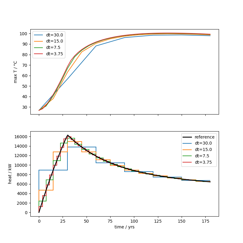
Let’s extract the temperature evolution and the applied heat via vtuIO and plot both:
time = np.append(0.0, np.geomspace(1.0, 180.0, num=100))
repo = physics.nuclearwasteheat.repo_2020_conservative
heat = repo.heat(time, time_unit="yrs", power_unit="kW")
fig, (ax1, ax2) = plt.subplots(figsize=(8, 8), nrows=2, sharex=True)
ax2.plot(time, heat, lw=2, label="reference", color="k")

for sim_result, dt in zip(sim_results, time_step_sizes, strict=False):
    ms = ot.MeshSeries(sim_result, time_unit="yrs")
    max_T = ot.variables.temperature.max.transform(ms)
    ax1.plot(ms.timevalues, max_T, lw=1.5, label=f"{dt=}")

    edges = np.append(0, ms.timevalues)
    mean_t = 0.5 * (edges[1:] + edges[:-1])
    applied_heat = repo.heat(mean_t, time_unit="yrs", power_unit="kW")
    ax2.stairs(applied_heat, edges, lw=1.5, label=f"{dt=}", baseline=None)
ax1.set(ylabel="max T / °C")
ax2.set(xlabel="time / yrs", ylabel="heat / kW")
ax1.legend()
ax2.legend()
fig.show()
Temperature convergence at maximum heat production (t=30 yrs)#
The grid convergence at this timepoint deviates significantly from 1, meaning the convergence is suboptimal (at least on the left boundary where the heating happens). The chosen timesteps are still to coarse to reach an asymptotic range of convergence. The model behavior at this early part of the simulation is still very dynamic and needs finer timesteps to be captured with great accuracy. Nevertheless, the maximum temperature converges quadratically, as expected.
report_name = temp_path / "report.ipynb"
studies.convergence.run_convergence_study(
    output_name=report_name,
    mesh_paths=sim_results,
    timevalue=30 * sec_per_yr,
    variable_name="temperature",
    refinement_ratio=2.0,
)
HTML(workflow.jupyter_to_html(report_name, show_input=False))
# SPDX-FileCopyrightText: Copyright (c) OpenGeoSys Community (opengeosys.org)
# SPDX-License-Identifier: BSD-3-Clause

# ---
# jupyter:
#   kernelspec:
#     display_name: .venv
#     language: python
#     name: python3
# ---
Grid convergence
If the shown values are approximately 1, this means that the results are in asymptotic range of convergence.

Grid comparison
Visualizing the requested mesh variable on the 3 finest discretizations:

Richardson extrapolation
Visualizing the Richardson extrapolation of the requested mesh variable. If a reference solution is provided, the difference between the two is shown as well. Otherwise the difference between the finest discretization and the Richardson extrapolation is shown.


Convergence metrics
Relative errors

Absolute values

Temperature convergence at maximum temperature (t=150 yrs)#
The temperature convergence at this timevalue is much closer to 1, indicating a better convergence behaviour, which is due to the temperature gradient now changing only slowly. Convergence order is again quadratic.
studies.convergence.run_convergence_study(
    output_name=report_name,
    mesh_paths=sim_results,
    timevalue=150 * sec_per_yr,
    variable_name="temperature",
    refinement_ratio=2.0,
)
HTML(workflow.jupyter_to_html(report_name, show_input=False))
# SPDX-FileCopyrightText: Copyright (c) OpenGeoSys Community (opengeosys.org)
# SPDX-License-Identifier: BSD-3-Clause

# ---
# jupyter:
#   kernelspec:
#     display_name: .venv
#     language: python
#     name: python3
# ---
Grid convergence
If the shown values are approximately 1, this means that the results are in asymptotic range of convergence.

Grid comparison
Visualizing the requested mesh variable on the 3 finest discretizations:

Richardson extrapolation
Visualizing the Richardson extrapolation of the requested mesh variable. If a reference solution is provided, the difference between the two is shown as well. Otherwise the difference between the finest discretization and the Richardson extrapolation is shown.


Convergence metrics
Relative errors

Absolute values

Convergence evolution over all timesteps#
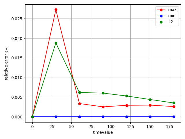
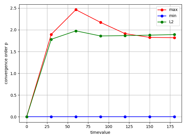
We can also run the convergence evaluation on all timesteps and look at the relative errors (between finest discretization and Richardson extrapolation) and the convergence order over time to get a better picture of the transient model behavior.
ms = [ot.MeshSeries(sim_result) for sim_result in sim_results]
evolution_metrics = studies.convergence.convergence_metrics_evolution(
    ms, ot.variables.temperature, units=["s", "yrs"]
)
  0%|          | 0/7 [00:00<?, ?it/s]
 43%|████▎     | 3/7 [00:00<00:00, 26.96it/s]
 86%|████████▌ | 6/7 [00:00<00:00, 25.59it/s]
100%|██████████| 7/7 [00:00<00:00, 25.61it/s]
Looking at the errors, we see a higher error right at the beginning. This is likely due to the more dynamic behavior at the beginning.
fig = studies.convergence.plot_convergence_error_evolution(
    evolution_metrics, error_type="absolute"
)
fig.show()
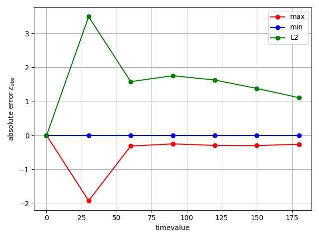
fig = studies.convergence.plot_convergence_error_evolution(
    evolution_metrics, error_type="relative"
)
fig.show()
A look at the convergence order evolution shows almost quadratic convergence over the whole timeframe. For the maximum temperature we even get better than quadratic behavior, which is coincidentally and most likely model dependent.
fig = studies.convergence.plot_convergence_order_evolution(evolution_metrics)
fig.show()
Total running time of the script: (0 minutes 29.382 seconds)
