Creating a BHE mesh (Borehole Heat Exchanger)

This example demonstrates how to create a Borehole Heat Exchanger (BHE) mesh.

import pyvista as pv
from shapely import Polygon

import ogstools as ot
from ogstools import examples
from ogstools.meshes.gmsh_BHE import BHE, Groundwater, gen_bhe_mesh

Introduction

This example shows the general usage of ogstools.meshes.gmsh_BHE.gen_bhe_mesh() and how some of the parameters will effect the mesh. This section demonstrates the mesh generation with only three soil layers, groundwater flow in one layer and three BHE’s. However, this tool provides multiple soil layers, groundwater flow in multiple layers and multiple BHE’s. The mesh sizes provides good initial values for the most Heat-Transport-BHE simulations in OGS. They can also be set by the user, to customize the mesh. Feel free to try it out!

Create a simple prism mesh

Generate a customizable prism BHE mesh:

bhe_meshes = gen_bhe_mesh(
    model_area=Polygon.from_bounds(xmin=0, ymin=0, xmax=150, ymax=100),
    layer=[50, 50, 50],
    groundwater=Groundwater(
        begin=-30,
        isolation_layer_id=1,
        upstream=(179, 181),
        downstream=(359, 1),
    ),
    BHE_Array=[
        BHE(x=50, y=40, z_begin=-1, z_end=-60, borehole_radius=0.076),
        BHE(x=50, y=50, z_begin=-1, z_end=-60, borehole_radius=0.076),
        BHE(x=50, y=60, z_begin=-1, z_end=-60, borehole_radius=0.076),
    ],
    refinement_area=Polygon.from_bounds(xmin=40, ymin=30, xmax=60, ymax=70),
    meshing_type="prism",
    meshname="bhe_prism",
)

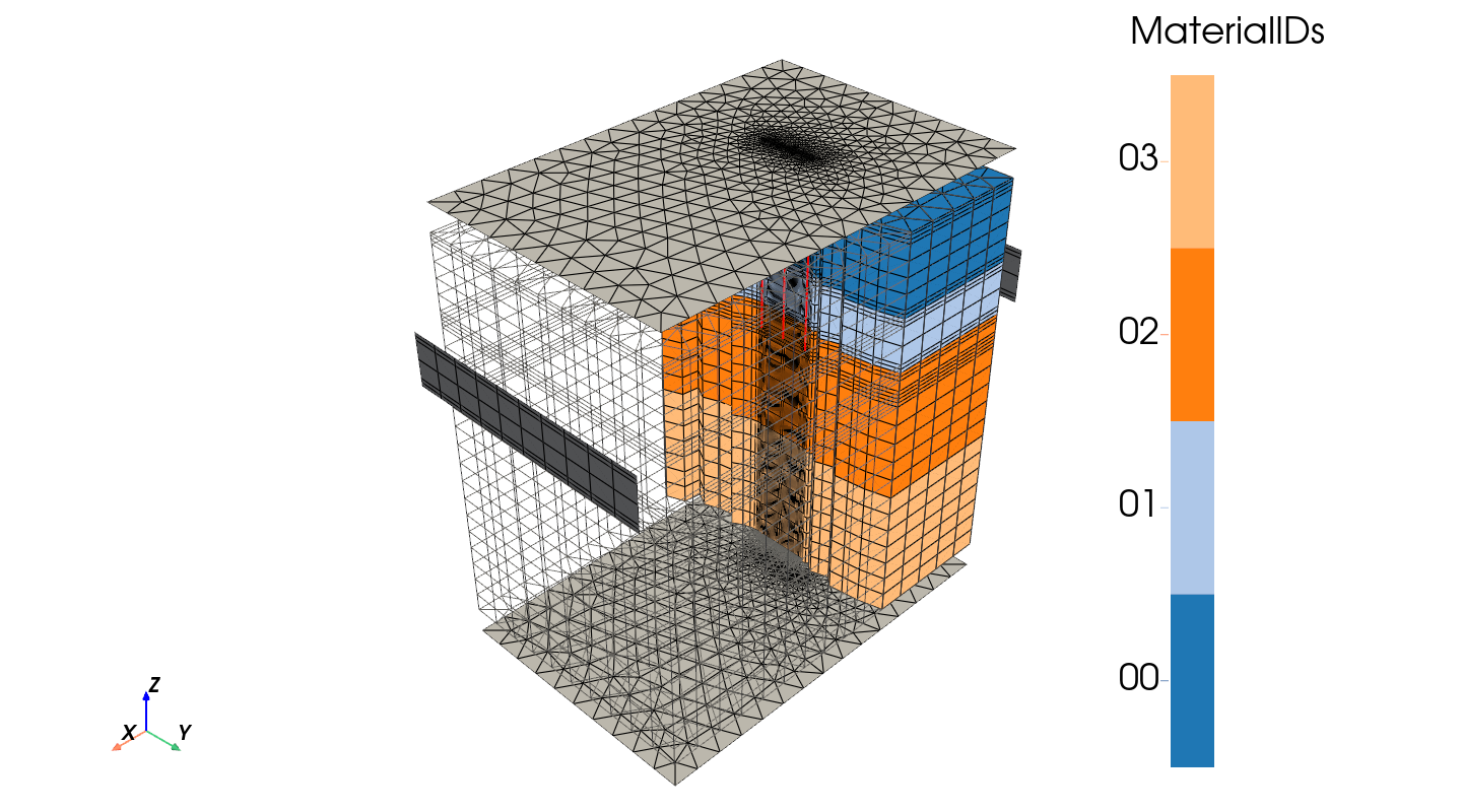
Load the domain mesh and all submeshes, extract the BHE lines and visualize it all:

def load_and_plot(bhe_meshes: ot.Meshes):
    bhe_line = bhe_meshes.domain.extract_cells_by_type(pv.CellType.LINE)
    offsets = [(0, 0, 10), (0, 0, -10), (10, 0, 0), (-10, 0, 0)]
    plotter = ot.plot.contourf(
        bhe_meshes.domain.clip("x", origin=bhe_line.center, crinkle=True),
        ot.variables.material_id,
    )
    plotter.add_mesh(bhe_meshes.domain, style="wireframe", color="grey")
    plotter.add_mesh(bhe_line, color="r", line_width=3)

    for submesh, offset in zip(
        bhe_meshes.subdomains.values(), offsets, strict=True
    ):
        plotter.add_mesh(
            submesh.translate(offset), show_edges=True, color="lightgrey"
        )
    plotter.show()

load_and_plot(bhe_meshes)

Static Scene

Interactive Scene

Create a simple structured mesh

Generate a customizable structured BHE mesh:

bhe_meshes = gen_bhe_mesh(
    model_area=Polygon.from_bounds(xmin=0, ymin=0, xmax=150, ymax=100),
    layer=[50, 50, 50],
    groundwater=Groundwater(
        begin=-30,
        isolation_layer_id=1,
        upstream=(179, 181),
        downstream=(359, 1),
    ),
    BHE_Array=[
        BHE(x=50, y=40, z_begin=-1, z_end=-60, borehole_radius=0.076),
        BHE(x=50, y=50, z_begin=-1, z_end=-60, borehole_radius=0.076),
        BHE(x=50, y=60, z_begin=-1, z_end=-60, borehole_radius=0.076),
    ],
    refinement_area=Polygon.from_bounds(xmin=40, ymin=30, xmax=60, ymax=70),
    meshing_type="structured",
    meshname="bhe_prism_2",
)

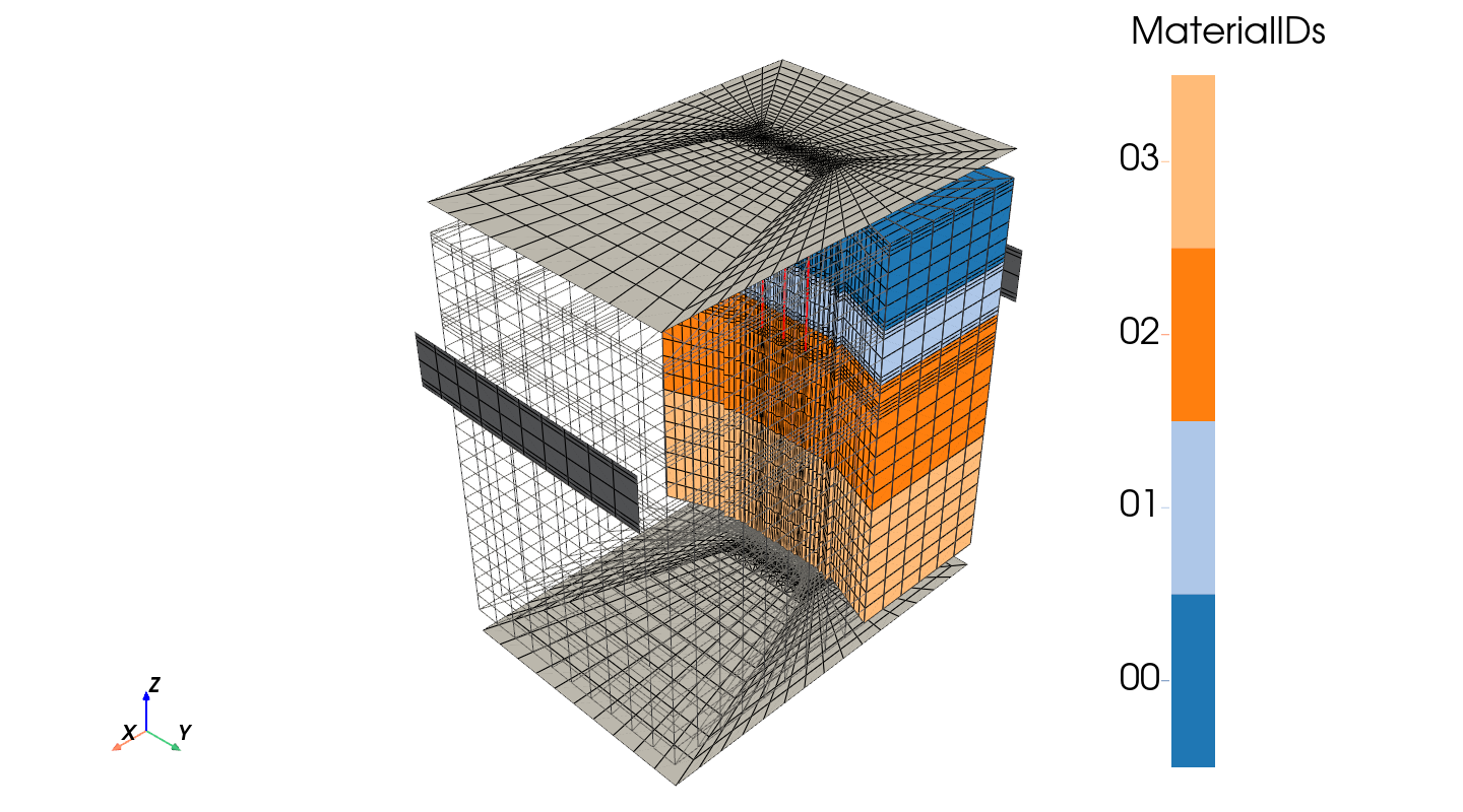
Load the domain mesh and all submeshes as well as extract the BHE lines:

load_and_plot(bhe_meshes)

Static Scene

Interactive Scene

Create an advanced structured mesh

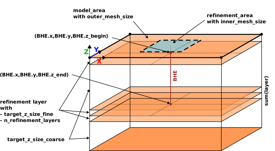
Generate a customizable structured BHE mesh with advanced mesh sizing options (using gmsh). By adding additional points to the model_area, the subdivison of the surface by the structured mesh algorithm is controlled. To understand the specific behaviour of every mesh parameter, test each one after another.

bhe_meshes = gen_bhe_mesh(
    # add additional points for better subsidivision of the surface by structured algorithm
    # compare with previous example, to see the difference
    model_area=Polygon(
        (
            (0.0, 0.0),
            (40.0, 0.0),
            (60.0, 0.0),
            (150.0, 0.0),
            (150.0, 100.0),
            (60.0, 100.0),
            (40.0, 100.0),
            (0.0, 100.0),
        )
    ),
    layer=[50, 50, 50],
    groundwater=Groundwater(
        begin=-30,
        isolation_layer_id=1,
        upstream=(179, 181),
        downstream=(359, 1),
    ),
    BHE_Array=[
        BHE(50, 40, -1, -60, 0.076),
        BHE(50, 50, -1, -60, 0.076),
        BHE(50, 60, -1, -60, 0.076),
    ],
    refinement_area=Polygon.from_bounds(xmin=40, ymin=30, xmax=60, ymax=70),
    meshing_type="structured",
    target_z_size_coarse=10,  # default value 7.5
    target_z_size_fine=2,  # default value 1.5
    n_refinement_layers=1,  # default value 2
    propagation=1.2,  # default value 1.1
    inner_mesh_size=8,  # default value 5
    outer_mesh_size=12,  # default value 10
    meshname="bhe_structured",
)

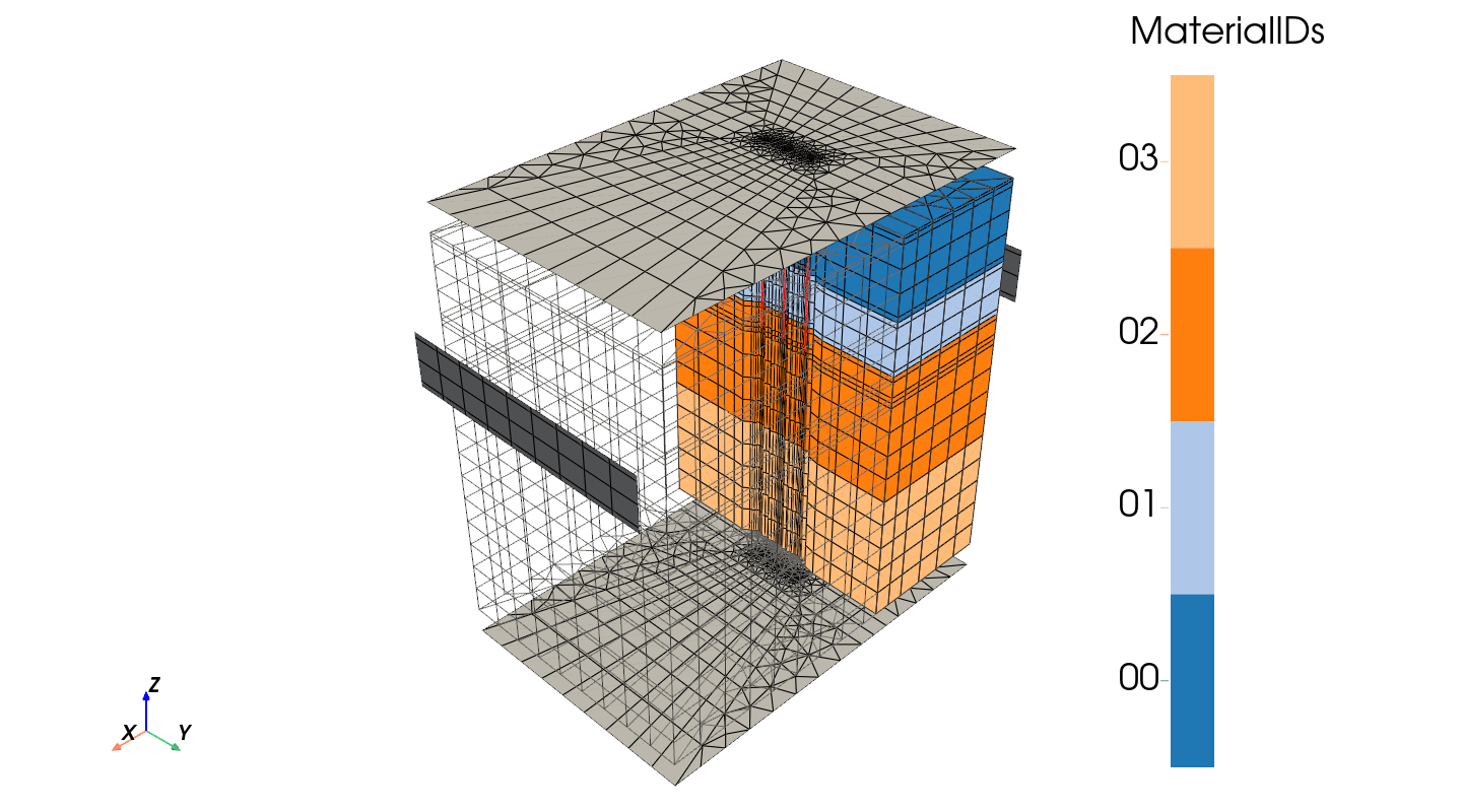
Load the domain mesh and all submeshes as well as extract the BHE lines:

load_and_plot(bhe_meshes)

Static Scene

Interactive Scene

Accessing simulated BHE temperatures

BHE simulation results store temperature per pipe instead of as a single vector. Which component names exist depends on the BHE type - a single U-tube (1U) has one pipe loop (in, out, grout1, grout2), while a double U-tube (2U) has two independent loops in the same borehole (in1/in2, out1/out2, grout1..``grout4``). Components_BHE (e.g. ot.variables.temperature_BHE) knows this per-type layout.

For a mesh with several boreholes, indexing takes a second, separate argument: the BHE number. E.g. in the mesh below, BHE 1 and 3 are 1U and BHE 2 is 2U. We probe the inflow temperature at the top of each borehole over time:

mesh_series = examples.load_meshseries_BHEs_3D("full", ".pvd")
bhe_tops = [(-6.0, 25.0, -27.0), (0.0, 25.0, -27.0), (6.0, 25.0, -27.0)]
mesh_series.probe_values(bhe_tops[0], ot.variables.temperature_BHE[1, "in"])
mesh_series.probe_values(bhe_tops[1], ot.variables.temperature_BHE[2, "in1"])
mesh_series.probe_values(bhe_tops[1], ot.variables.temperature_BHE[2, "in2"])

  0%|          | 0/2 [00:00<?, ?it/s]
100%|██████████| 2/2 [00:00<00:00, 453.41it/s]

array([21.85      , 22.10904858])