

Note
Go to the end to download the full example code or to run this example in your browser via Binder.
Spatial refinement - steady state diffusion#
This example shows one possible implementation of how to do a convergence study. It uses the project file from the following benchmark with multiple discretizations to evaluate the accuracy of the numerical solutions. ogs: elliptic neumann benchmark
Here is some theoretical background for the topic of grid convergence:
At least three meshes of increasing refinement are required for the convergence study. The three finest meshes are used to calculated the Richardson extrapolation. The third coarsest mesh will be used for the topology to evaluate the results. Its nodes should be shared by the finer meshes, otherwise interpolation will influence the results. With unstructured grids this can be achieved as well with refinement by splitting.
The results to analyze are generated on the fly with the following code. If you are only interested in the convergence study, please skip to Hydraulic pressure convergence.
First, the required packages are imported and an output directory is created:
from IPython.display import HTML

import ogstools as ot
from ogstools import examples, workflow
from ogstools.studies import convergence

tmp_path = ot.definitions.temp_dir("steady_state_diffusion", "examples")
report_name = str(tmp_path / "report.ipynb")
The meshes and their boundaries are generated easily via gmsh and
Meshes. from_gmsh().
Then we run the different simulations with increasingly fine spatial
discretization via ogs6py and store the results for the convergence study.
refinements = 6
edge_cells = [2**i for i in range(refinements)]
simulations_control = []

for n_edge_cells in edge_cells:
    meshes = ot.Meshes.from_gmsh(
        ot.gmsh_tools.rect(n_edge_cells=n_edge_cells, structured_grid=True),
        log=False,
    )

    prj = ot.Project(input_file=examples.prj_steady_state_diffusion).copy(
        tmp_path / f"cells_{n_edge_cells}"
    )
    prefix = "steady_state_diffusion_" + str(n_edge_cells)
    prj.replace_text(prefix, ".//prefix")

    model = ot.Model(prj, meshes)
    sim_c = model.controller()
    simulations_control.append(sim_c)

simulations = [sim.run() for sim in simulations_control]
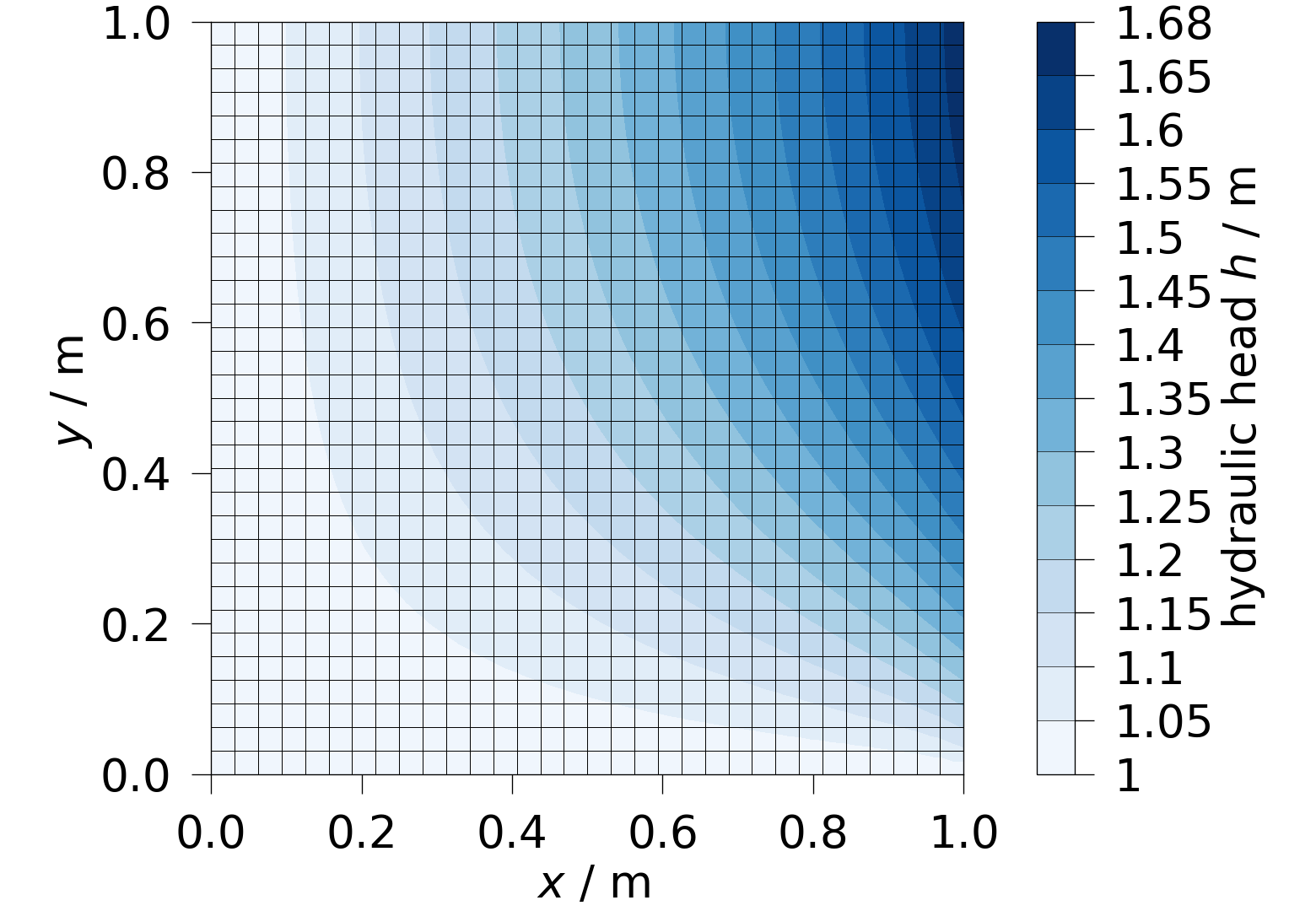
Here we calculate the analytical solution on one of the meshes:
analytical_solution_path = tmp_path / "analytical_solution.vtu"
sim_last: ot.Simulation = simulations[-1]

solution = examples.anasol.diffusion_head_analytical(
    simulations[-1].meshseries[0]
)
ot.plot.setup.show_element_edges = True
fig = ot.plot.contourf(solution, ot.variables.hydraulic_head)
fig.show()
analytical_solution_path = ot.mesh.save(solution)
Hydraulic pressure convergence#
The pressure field of this model is converging well. The convergence ratio is approximately 1 on the whole mesh and looking at the relative errors we see a quadratic convergence behavior.
result_paths = [sim.meshseries_file for sim in simulations]
convergence.run_convergence_study(
    output_name=report_name,
    mesh_paths=result_paths,
    variable_name="hydraulic_head",
    timevalue=1,
    refinement_ratio=2.0,
    reference_solution_path=str(analytical_solution_path),
)
HTML(workflow.jupyter_to_html(report_name, show_input=False))
# SPDX-FileCopyrightText: Copyright (c) OpenGeoSys Community (opengeosys.org)
# SPDX-License-Identifier: BSD-3-Clause

# ---
# jupyter:
#   kernelspec:
#     display_name: .venv
#     language: python
#     name: python3
# ---
Grid convergence
If the shown values are approximately 1, this means that the results are in asymptotic range of convergence.

Grid comparison
Visualizing the requested mesh variable on the 3 finest discretizations:

Richardson extrapolation
Visualizing the Richardson extrapolation of the requested mesh variable. If a reference solution is provided, the difference between the two is shown as well. Otherwise the difference between the finest discretization and the Richardson extrapolation is shown.


Convergence metrics
Relative errors

Absolute values

Darcy velocity convergence#
For the velocity we some discrepancy of the convergence ratio in the bottom right corner. Thus we know, at these points the mesh isn’t properly converging (at least for the velocity field). We see, that in the bottom right corner, the velocity magnitude seems to be steadily increasing, which is also reflected in the Richardson extrapolation, which shows an anomalous high value in this spot, hinting at a singularity there. This is explained by the notion in the benchmark’s documentation of “incompatible boundary conditions imposed on the bottom right corner of the domain.” Regardless of this, the benchmark gives a convergent solution for the pressure field. The code cells from the templated notebook are show here for transparency.
convergence.run_convergence_study(
    output_name=report_name,
    mesh_paths=result_paths,
    variable_name="velocity",
    timevalue=1,
    refinement_ratio=2.0,
)
HTML(workflow.jupyter_to_html(report_name, show_input=True))
# SPDX-FileCopyrightText: Copyright (c) OpenGeoSys Community (opengeosys.org)
# SPDX-License-Identifier: BSD-3-Clause

# ---
# jupyter:
#   kernelspec:
#     display_name: .venv
#     language: python
#     name: python3
# ---
# Import required modules and customize plot settings.
# pylint:disable=C0413
import numpy as np
import pyvista as pv
from IPython.display import display

import ogstools as ot
from ogstools import studies

ot.plot.setup.reset()
ot.plot.setup.show_element_edges = True
ot.plot.setup.combined_colorbar = False


def _show_with_alt(fig: object, alt: str) -> None:
    """Display a matplotlib figure with alt text, then close it."""
    if isinstance(fig, ot.plot.contourplots.plt.Figure):
        display(fig, metadata={"image/png": {"alt": alt}})
        ot.plot.contourplots.plt.close(fig)
# Here, the meshes are read, a Variable object is created from the variable
# name and the Richardson extrapolation calculated.
# The 3 finest meshes of those provided will be used for the Richardson
# extrapolation.

mesh_series = [ot.MeshSeries(mesh_path) for mesh_path in mesh_paths]
timestep_sizes = [np.mean(np.diff(ms.timevalues)) for ms in mesh_series]
meshes = [ms.mesh(ms.closest_timestep(timevalue)) for ms in mesh_series]
topology: pv.UnstructuredGrid = meshes[-3]
variable = ot.variables.Variable.find(variable_name, meshes[0])
richardson = studies.convergence.richardson_extrapolation(
    meshes, variable, topology, refinement_ratio
)
Grid convergence
If the shown values are approximately 1, this means that the results are in asymptotic range of convergence.

Grid comparison
Visualizing the requested mesh variable on the 3 finest discretizations:

Richardson extrapolation
Visualizing the Richardson extrapolation of the requested mesh variable. If a reference solution is provided, the difference between the two is shown as well. Otherwise the difference between the finest discretization and the Richardson extrapolation is shown.
fig = ot.plot.contourf(richardson, variable)
_show_with_alt(
    fig,
    f"Contour plot of the Richardson extrapolation of {variable.output_name}.",
)

data_key = variable.data_name
if reference_solution_path is None:
    diff_mesh = ot.mesh.difference(
        richardson, topology.sample(meshes[-1]), variable
    )
    fig = ot.plot.contourf(diff_mesh, variable)
    _show_with_alt(
        fig,
        f"Contour plot of the difference in {variable.output_name} between "
        "the finest discretization and the Richardson extrapolation.",
    )
else:
    ms = ot.MeshSeries(reference_solution_path)
    timestep = ms.closest_timestep(timevalue)
    reference_solution = topology.sample(ms.mesh(timestep))
    diff_mesh = ot.mesh.difference(reference_solution, richardson, variable)
    fig = ot.plot.contourf(diff_mesh, variable)
    _show_with_alt(
        fig,
        f"Contour plot of the difference in {variable.output_name} between "
        "the reference solution and the Richardson extrapolation.",
    )


Convergence metrics
metrics = studies.convergence.convergence_metrics(
    meshes, richardson, variable, timestep_sizes
)
metrics.style.format("{:,.5g}").hide()
Relative errors

Absolute values

Total running time of the script: (0 minutes 17.295 seconds)
