OGSTools Framework - Complete Workflow Guide

This guide demonstrates the complete OGSTools workflow for setting up, running, and analyzing OpenGeoSys (OGS) simulations. It helps to get an overview of how the different components work together.

Workflow Overview

1. Setup: Load or create Project files and Meshes

2. Compose: Combine components into a Model with Execution settings

3. Run: Execute simulations and get Results

4. Analyze: Visualize and examine simulation outputs

5. Store: Save and reload simulation data for later use

For detailed information on each component, see the linked examples throughout this guide.

import tempfile
from pathlib import Path

import numpy as np

import ogstools as ot
from ogstools.examples import load_meshes_simple_lf, load_project_simple_lf

1. Setup: Project Files and Meshes

The first step is to prepare your simulation inputs. OGSTools provides two main components for this:

• Project Files (Project): Contains the simulation configuration (process type, parameters, boundary conditions, etc.) based on OGS .prj files (XML-format).

• Meshes (Meshes): Contains the computational domain geometry and mesh data. Can include multiple meshes (domain + boundary meshes).

For this example, we load pre-configured components.

project = load_project_simple_lf()
meshes = load_meshes_simple_lf()

In practice, you would:

• Create Project files programmatically: See How to Create Simple Mechanics Problem

• Generate meshes (with GMSH, Pyvista or similar): See Meshes from gmsh (msh2vtu), Extracting boundaries of a 2D mesh

Understanding Meshes: Input Geometry with PyVista

Meshes is the input mesh for OGS. Technically it is a collection of PyVista Unstructured grids that represent your simulation domain. You can access and manipulate individual meshes:

# Access a specific boundary mesh
print(f"Available meshes: {list(meshes.keys())}")

# Meshes are PyVista objects - The example shows how you can set initial conditions or properties
meshes["right"].point_data["pressure"] = np.full(meshes["left"].n_points, 3.1e7)

# Visualize the mesh topology
fig_topology = meshes.plot()

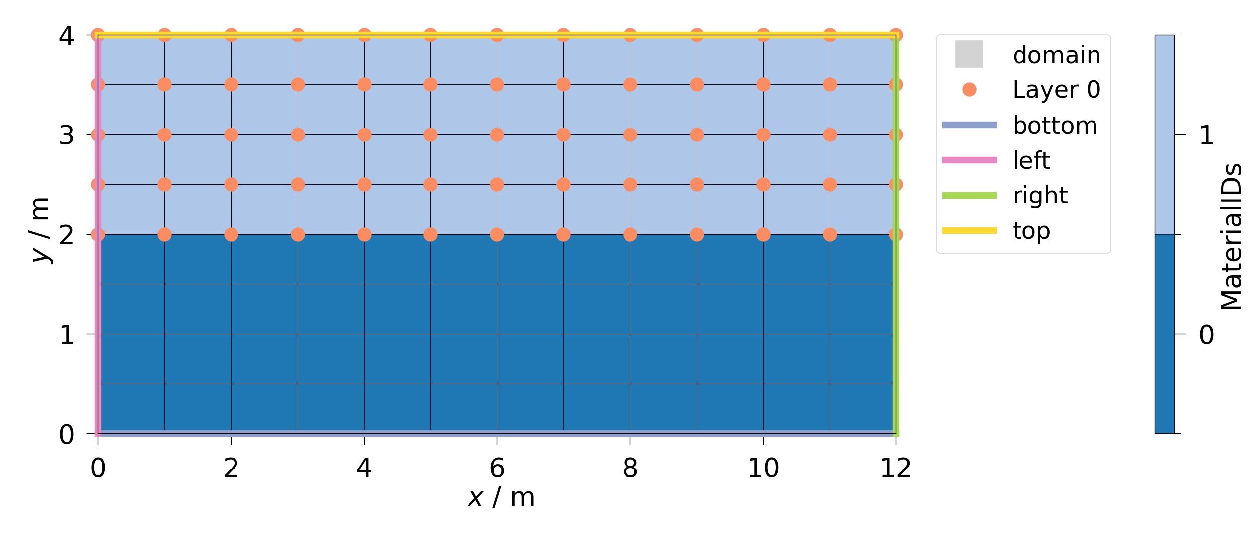
Available meshes: ['domain', 'bottom', 'top', 'right', 'left', 'Layer 0']

See also:

• Creating meshes from vtu surface files - Load meshes from VTU files

• Setting initial properties and variables in bulk meshes - Set initial conditions

2. Compose a Model

A Model combines all components needed to run a simulation:

• project: The simulation configuration (Project)

• meshes: The computational meshes (Meshes)

• execution: Runtime settings (Execution)

The Execution object controls how OGS runs (threads, MPI ranks, logging, etc.):

model = ot.Model(project=project, meshes=meshes)

# Optionally configure execution settings
# e.g. model.execution.interactive = True # Uncomment for stepwise control

# Visualize the model setup with boundary conditions
fig_constraints = model.plot_constraints()

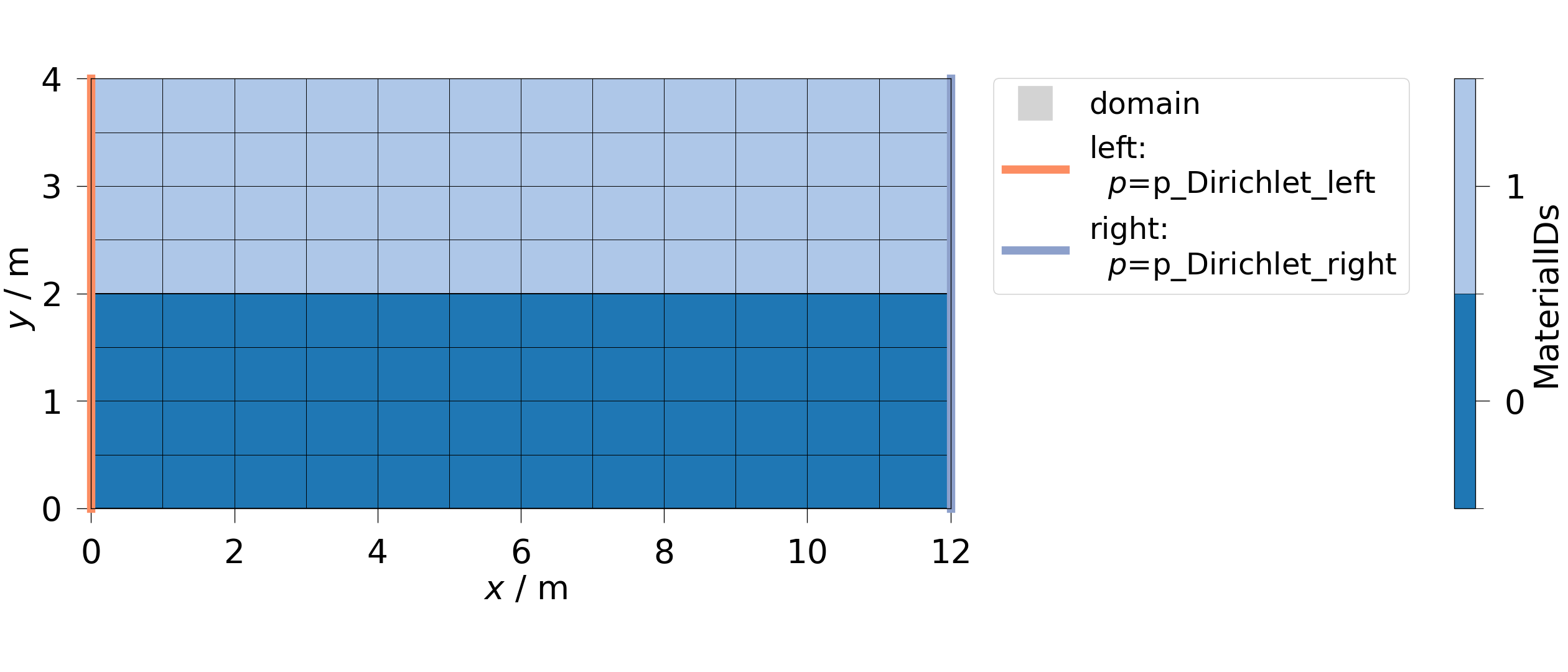
The constraints plot shows your model domain with annotated boundary conditions and source terms, making it easy to verify your setup before running.

3. Run: Execute the Simulation

OGSTools provides two ways to run simulations:

Option 1: Direct run (used here)

model.run() - Blocks until completion, returns Simulation

Option 2: Controlled execution

controller = model.controller() - Returns a SimulationController for monitoring

The controller approach gives you fine-grained control over execution.

See also: Run a simulation

controller = model.controller()
# Monitor status
print(controller.status_str)
# Run to wait for completion
sim = controller.run()

# Check simulation status
print(f"Simulation status: {sim.status_str}")

<bound method OGSNativeController.status_str of Model.from_folder('/tmp/ogstools_root/Model/20260323_113650_653601').controller(sim_output='/tmp/ogstools_root/Result/20260323_113651_008918', overwrite=True)
meshseries_file='/tmp/ogstools_root/Result/20260323_113651_008918/LiquidFlow_Simple.pvd'
logfile='/tmp/ogstools_root/Result/20260323_113651_008918/log.txt'
status=Status: running for 0.0003101825714111328 s.
execution.interactive=False>
Simulation status: Status: completed successfully (results available)

The Simulation object contains:

• model: The Model that was run

• result: Link to output files (MeshSeries)

• log: Parsed simulation log for analysis

• status: Completion status (derived from log analysis)

4. Analyze: Visualize and Examine Results

After simulation, you can analyze results using two main components:

MeshSeries (MeshSeries)

Access simulation results at different timesteps for visualization.

Log (Log)

Parse and analyze the simulation log (convergence, timing, errors).

Visualizing Results with MeshSeries

The sim.result property provides a MeshSeries interface to your output data. You can index it like a list to get results at specific timesteps:

# Get the final timestep and plot pressure distribution
fig = ot.plot.contourf(sim.meshseries[-1], "pressure")

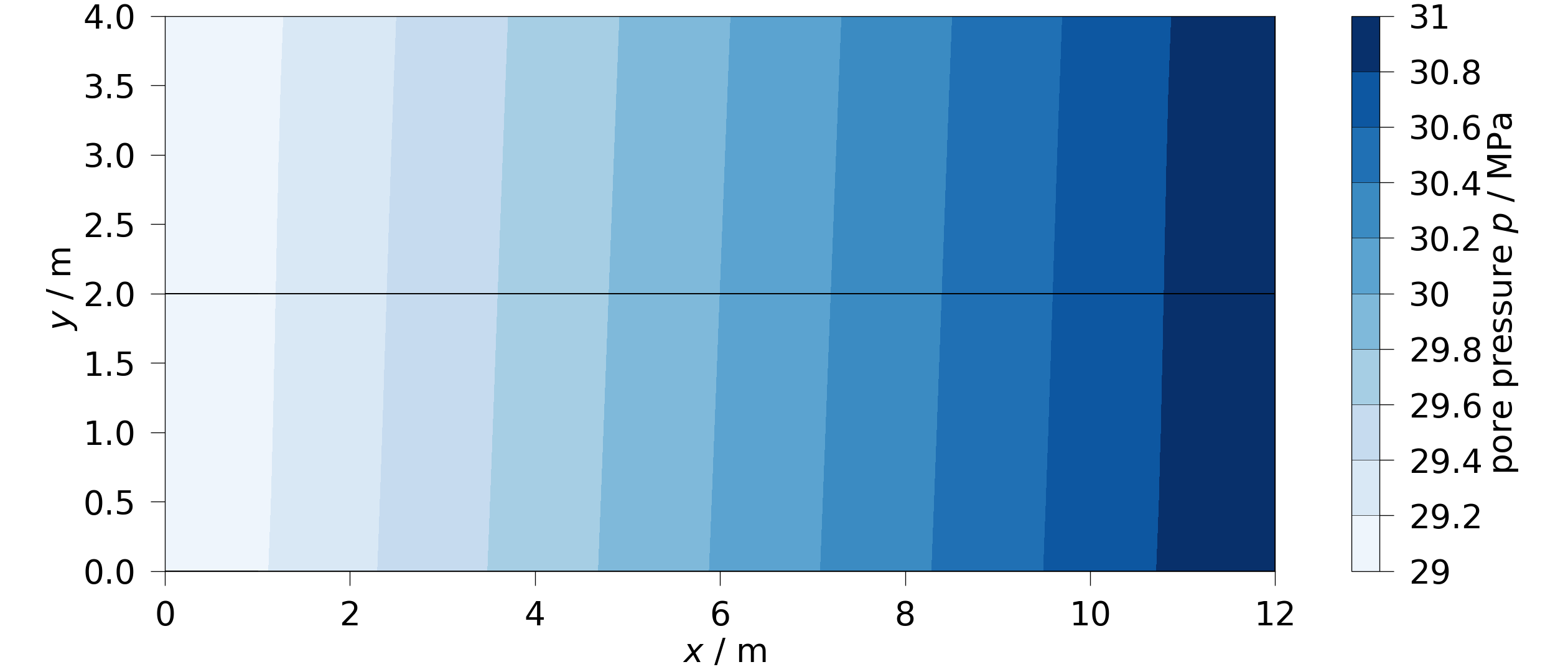
MeshSeries capabilities:

• Access any timestep: sim.result[0], sim.result[-1]

• Iterate over time: for mesh in sim.result: ...

• Time slicing: sim.result[::10] (every 10th timestep)

• Unit conversion: sim.result.scale(time="h", length="cm")

See also:

• Read mesh from file (vtu or xdmf) into pyvista mesh - Detailed MeshSeries tutorial

• Visualizing 2D model data - 2D visualization options

• Visualizing 3D model data - 3D visualization options

• How to create Animations - Create time animations

Analyzing Convergence with the Log Parser

The log parser extracts convergence data, timestep information, and errors from the simulation log file:

# Plot simulation time
df_ts = ot.logparser.analysis_time_step(sim.log.df_log).reset_index()
times = ["assembly_time", "dirichlet_time", "linear_solver_time"]
df_ts.plot.area(x="time_step", y=times, ylabel="time / s", grid=True)

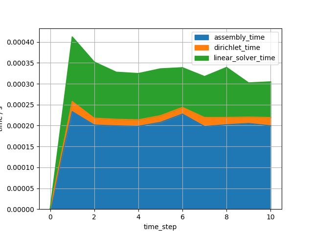
<Axes: xlabel='time_step', ylabel='time / s'>

The convergence plot shows how the nonlinear solver converged at each time step, helping you identify potential numerical issues.

Log analysis capabilities:

• Convergence data: sim.log.convergence_newton_iteration()

• Time step info: sim.log.time_step()

• Termination status: sim.log.simulation_termination()

• Custom plots: sim.log.plot_convergence(metric="dx", x_metric="model_time")

See also:

• Logparser: Introduction - Log parser introduction

• Logparser: Predefined Analyses - Analysis examples

• Logparser: Advanced topics - Advanced log parsing

5. Store: Save and Reload Simulations

OGSTools provides a unified storage system for saving complete simulations (or individual components) for later analysis or sharing.

Key features:

• Cascading save: Saving a Simulation automatically saves Model and Results

• Archive mode: Create self-contained copies (no symlinks)

• ID-based organization: Use IDs for organized storage

• Complete roundtrip: Save → load → identical object

tmp = Path(tempfile.mkdtemp())

# Save the complete simulation with archive mode
# This creates a self-contained copy you can share or move
sim.save(tmp / "mysim", archive=True)
# The saved simulation can be loaded later for further investigation

[]